Using ecco_access in Jupyter notebooks and Python code

Introduction

Importing ecco_access to your workspace

The ecco_podaac_to_xrdataset function

The ecco_podaac_access function

Introduction

In the past several years since ECCOv4 release 4 output was made available on the Physical Oceanography Distributed Active Archive Center or PO.DAAC, a number of Python scripts/functions have been written to facilitate requests of this output, authored by Jack McNelis, Ian Fenty, and Andrew Delman. These codes have been consolidated into the ecco_access package, in order to standardize the format of the requests.

This tutorial will help you to start using the two top-level functions in the ecco_access Python package:

• ecco_podaac_to_xrdataset: takes as input a text query or ECCO dataset identifier, and returns an xarray Dataset

• ecco_podaac_access: takes the same input, but returns the URLs/paths or local files where the data is located

Importing ecco_access to your workspace

After you have installed the ecco_access package, you can import it into your Python code and notebooks to use its functions:

import ecco_access as ea

Find any bugs?

If you installed a recent version of ecco_access using conda install ecco_access or pip install ecco_access and you are encountering errors, please reach out to andrewdelman@ucla.edu. You can also try cloning the ECCO-ACCESS Github repository that contains ecco_access code, as the Github repository may have bug fixes that have not been pushed to conda-forge or pypi yet. Then add the repository to the beginning of your Python path by putting the following code in your notebooks:

import sys
sys.path.insert(0,'path/to/ECCO-ACCESS')
import ecco_access as ea

Note: From April to October 2025, the ecco_access modules were included in the ecco_v4_py Python package (e.g., version 1.7.8). Starting in October 2025, these modules are available in the standalone ecco_access package. If using an ecco_v4_py release that has these modules, you should be able to use the functions below by calling import ecco_v4_py.ecco_access as ea. Going forward, these functions will not be inclued in ecco_v4_py, only in the ecco_access package.

The ecco_podaac_to_xrdataset function

Perhaps the most convenient way to use ecco_access is the ecco_podaac_to_xrdataset; it takes as input a query consisting of NASA Earthdata dataset ShortName(s), ECCO variables, or text strings in the variable descriptions, and outputs an xarray Dataset. Let’s look at the syntax:

import xarray as xr
import matplotlib.pyplot as plt
from os.path import join,expanduser

import ecco_v4_py as ecco
import ecco_access as ea

# identify user's home directory
user_home_dir = expanduser('~')

help(ea.ecco_podaac_to_xrdataset)

Help on function ecco_podaac_to_xrdataset in module ecco_access.ecco_access:

ecco_podaac_to_xrdataset(query, version='v4r4', grid=None, time_res='all', StartDate=None, EndDate=None, snapshot_interval=None, mode='download_ifspace', download_root_dir=None, **kwargs)
    This function queries and accesses ECCO datasets from PO.DAAC. The core query and download functions
    are adapted from Jupyter notebooks created by Jack McNelis and Ian Fenty
    (https://github.com/ECCO-GROUP/ECCO-ACCESS/blob/master/PODAAC/Downloading_ECCO_datasets_from_PODAAC/README.md)
    and modified by Andrew Delman (https://ecco-access.readthedocs.io).
    It is similar to ecco_podaac_access, except instead of a list of URLs or files,
    an xarray Dataset with all of the queried ECCO datasets is returned.

    Parameters
    ----------
    query: str, list, or dict, defines datasets or variables to access.
           If query is str, it specifies either a dataset ShortName (if query
           matches a NASA Earthdata ShortName), or a text string that can be
           used to search the ECCO ShortNames, variable names, and descriptions.
           A query may also be a list of multiple ShortNames and/or text searches,
           or a dict that contains grid,time_res specifiers as keys and ShortNames
           or text searches as values, e.g.,
           {'native,monthly':['ECCO_L4_SSH_LLC0090GRID_MONTHLY_V4R4',
                              'THETA']}
           will query the native grid monthly SSH datasets, and all native grid
           monthly datasets with variables or descriptions matching 'THETA'.

    version: ('v4r4','v4r5'), specifies ECCO version to query.
             Currently 'v4r5' only works with ['s3_open','s3_get','s3_get_ifspace'] modes,
             or if the files are already stored in download_root_dir/ShortName/.
             Otherwise an error is returned.

    grid: ('native','latlon',None), specifies whether to query datasets with output
          on the native grid or the interpolated lat/lon grid.
          The default None will query both types of grids, unless specified
          otherwise in a query dict (e.g., the example above).

    time_res: ('monthly','daily','snapshot','all'), specifies which time resolution
              to include in query and downloads. 'all' includes all time resolutions,
              and datasets that have no time dimension, such as the grid parameter
              and mixing coefficient datasets.


    StartDate,EndDate: str, in 'YYYY', 'YYYY-MM', or 'YYYY-MM-DD' format,
                       define date range [StartDate,EndDate] for download.
                       EndDate is included in the time range (unlike typical Python ranges).
                       Full ECCOv4r4 date range (default) is '1992-01-01' to '2017-12-31'.
                       For 'SNAPSHOT' datasets, an additional day is added to EndDate to enable
                       closed budgets within the specified date range.

    snapshot_interval: ('monthly', 'daily', or None), if snapshot datasets are included in ShortNames,
                       this determines whether snapshots are included for only the beginning/end
                       of each month ('monthly'), or for every day ('daily').
                       If None or not specified, defaults to 'daily' if any daily mean ShortNames
                       are included and 'monthly' otherwise.

    mode: str, one of the following:
          'download': Download datasets using NASA Earthdata URLs
          'download_ifspace': Check storage availability before downloading.
                              Download only if storage footprint of downloads
                              <= max_avail_frac*(available storage)
          'download_subset': Download spatial and temporal subsets of datasets
                             via Opendap; query help(ecco_access.ecco_podaac_download_subset)
                             to see keyword arguments that can be used in this mode.
          The following modes work within the AWS cloud only:
          's3_open': Access datasets on S3 without downloading.
          's3_open_fsspec': Use json files (generated with `fsspec` and `kerchunk`)
                            for expedited opening of datasets.
          's3_get': Download from S3 (to AWS EC2 instance).
          's3_get_ifspace': Check storage availability before downloading;
                            download if storage footprint
                            <= max_avail_frac*(available storage).
                            Otherwise data are opened "remotely" from S3 bucket.

    download_root_dir: str, defines parent directory to download files to.
                       Files will be downloaded to directory download_root_dir/ShortName/.
                       If not specified, parent directory defaults to '~/Downloads/ECCO_V4r4_PODAAC/',
                       or '~/Downloads/ECCO_V4r5_PODAAC/' if version == 'v4r5'.

    Additional keyword arguments*:
    *This is not an exhaustive list, especially for
    'download_subset' mode; use help(ecco_access.ecco_podaac_download_subset) to display
    options specific to that mode

    max_avail_frac: float, maximum fraction of remaining available disk space to
                    use in storing ECCO datasets.
                    If storing the datasets exceeds this fraction, an error is returned.
                    Valid range is [0,0.9]. If number provided is outside this range, it is replaced
                    by the closer endpoint of the range.

    jsons_root_dir: str, for s3_open_fsspec mode only, the root/parent directory where the
                    fsspec/kerchunk-generated jsons are found.
                    jsons are generated using the steps described here:
                    https://medium.com/pangeo/fake-it-until-you-make-it-reading-goes-netcdf4-data-on-aws-s3
                    as-zarr-for-rapid-data-access-61e33f8fe685.
                    If None (default), jsons_root_dir will be set to ~/MZZ/{version}/.
                    The jsons need to be stored in the following directories/formats:
                    For v4r4: {jsons_root_dir}/MZZ_{GRIDTYPE}_{TIME_RES}/{SHORTNAME}.json.
                    GRIDTYPE is '05DEG' or 'LLC0090GRID' for v4r4;
                    TIME_RES is one of: ('MONTHLY','DAILY','SNAPSHOT','GEOMETRY','MIXING_COEFFS').
                    For v4r5: {jsons_root_dir}/MZZ_{TIME_RES}_{GRIDTYPE}/{SHORTNAME_core}_{TIME_RES}_{GRIDTYPE}_llc090_ECCOV4r5.json.
                    TIME_RES is one of: ('mon_mean','day_mean','snap');
                    GRIDTYPE is one of: ('native','latlon').
                    The SHORTNAME_core is the SHORTNAME without the 'ECCO_L4_' at the beginning,
                    or the grid/time/version IDs at the end (e.g., 'LLC0090GRID_MONTHLY_V4R5').

    jsons_retrieve: bool, if True (default), and jsons are not already stored in jsons_root_dir,
                    retrieve from S3 bucket and store locally in jsons_root_dir.
                    If False, and jsons are not stored in jsons_root_dir,
                    the data retrieval will fail.

    n_workers: int, number of workers to use in concurrent downloads. Benefits typically taper off above 5-6.

    force_redownload: bool, if True, existing files will be redownloaded and replaced;
                            if False (default), existing files will not be replaced.

    show_noredownload_msg: bool, if True (default), and force_redownload=False,
                               display message for each file that is already
                               downloaded (and therefore not re-downloaded);
                               if False, these messages are not shown.

    prompt_request_payer: bool, if True (default), user is prompted to approve
                                (by entering "y" or "Y") any access to a
                                requester pays bucket, otherwise request is canceled;
                                if False, data access proceeds without prompting.

    Returns
    -------
    ds_out: xarray Dataset or dict of xarray Datasets (with ShortNames as keys),
            containing all of the accessed datasets.
            This function does not work with the query modes: 'ls','query','s3_ls','s3_query'.

There are a lot of options that you can use to “submit” a query with this function. Let’s consider a simple case, where we already have the ShortName for the monthly native grid SSH from ECCOv4r4 (ECCO_L4_SSH_LLC0090GRID_MONTHLY_V4R4), and we want to access output from the year 2017. The ShortName goes in the query field, and we can specify start and end dates (in YYYY-MM or YYYY-MM-DD format). The other options that matter most for this request are the mode, and depending on the mode, the download_root_dir or the jsons_root_dir.

Direct download over the internet (mode = ‘download’)

Let’s try the download mode, which retrieves the data over the Internet using NASA Earthdata URLs (this should work on any machine with Internet access, including cloud environments):

# download data and open xarray dataset
curr_shortname = 'ECCO_L4_SSH_LLC0090GRID_MONTHLY_V4R4'
ds_SSH = ea.ecco_podaac_to_xrdataset(curr_shortname,\
                                        StartDate='2017-01',EndDate='2017-12',\
                                        mode='download',\
                                        download_root_dir=join(user_home_dir,'Downloads','ECCO_V4r4_PODAAC'))

Creating download directory /home/jpluser/Downloads/ECCO_V4r4_PODAAC/ECCO_L4_SSH_LLC0090GRID_MONTHLY_V4R4
DL Progress: 100%|#########################| 12/12 [00:05<00:00,  2.16it/s]

=====================================
total downloaded: 71.02 Mb
avg download speed: 12.74 Mb/s
Time spent = 5.575884103775024 seconds

We specified a root directory for the download (which also happens to be the default setting), and the data files are then placed under download_root_dir / ShortName. We can verify that the contents of the file are what we queried:

ds_SSH

<xarray.Dataset> Size: 25MB
Dimensions:    (time: 12, tile: 13, j: 90, i: 90, i_g: 90, j_g: 90, nv: 2, nb: 4)
Coordinates: (12/13)
  * i          (i) int32 360B 0 1 2 3 4 5 6 7 8 9 ... 81 82 83 84 85 86 87 88 89
  * i_g        (i_g) int32 360B 0 1 2 3 4 5 6 7 8 ... 81 82 83 84 85 86 87 88 89
  * j          (j) int32 360B 0 1 2 3 4 5 6 7 8 9 ... 81 82 83 84 85 86 87 88 89
  * j_g        (j_g) int32 360B 0 1 2 3 4 5 6 7 8 ... 81 82 83 84 85 86 87 88 89
  * tile       (tile) int32 52B 0 1 2 3 4 5 6 7 8 9 10 11 12
  * time       (time) datetime64[ns] 96B 2017-01-16T12:00:00 ... 2017-12-16T0...
    ...         ...
    YC         (tile, j, i) float32 421kB dask.array<chunksize=(13, 90, 90), meta=np.ndarray>
    XG         (tile, j_g, i_g) float32 421kB dask.array<chunksize=(13, 90, 90), meta=np.ndarray>
    YG         (tile, j_g, i_g) float32 421kB dask.array<chunksize=(13, 90, 90), meta=np.ndarray>
    time_bnds  (time, nv) datetime64[ns] 192B dask.array<chunksize=(1, 2), meta=np.ndarray>
    XC_bnds    (tile, j, i, nb) float32 2MB dask.array<chunksize=(13, 90, 90, 4), meta=np.ndarray>
    YC_bnds    (tile, j, i, nb) float32 2MB dask.array<chunksize=(13, 90, 90, 4), meta=np.ndarray>
Dimensions without coordinates: nv, nb
Data variables:
    SSH        (time, tile, j, i) float32 5MB dask.array<chunksize=(1, 13, 90, 90), meta=np.ndarray>
    SSHIBC     (time, tile, j, i) float32 5MB dask.array<chunksize=(1, 13, 90, 90), meta=np.ndarray>
    SSHNOIBC   (time, tile, j, i) float32 5MB dask.array<chunksize=(1, 13, 90, 90), meta=np.ndarray>
    ETAN       (time, tile, j, i) float32 5MB dask.array<chunksize=(1, 13, 90, 90), meta=np.ndarray>
Attributes: (12/57)
    acknowledgement:              This research was carried out by the Jet Pr...
    author:                       Ian Fenty and Ou Wang
    cdm_data_type:                Grid
    comment:                      Fields provided on the curvilinear lat-lon-...
    Conventions:                  CF-1.8, ACDD-1.3
    coordinates_comment:          Note: the global 'coordinates' attribute de...
    ...                           ...
    time_coverage_duration:       P1M
    time_coverage_end:            2017-02-01T00:00:00
    time_coverage_resolution:     P1M
    time_coverage_start:          2017-01-01T00:00:00
    title:                        ECCO Sea Surface Height - Monthly Mean llc9...
    uuid:                         a21a5c30-400c-11eb-a9e0-0cc47a3f49c3

xarray.Dataset

• Dimensions:
  • time: 12
  • tile: 13
  • j: 90
  • i: 90
  • i_g: 90
  • j_g: 90
  • nv: 2
  • nb: 4
• Coordinates: (13)
  • i
    (i)
    int32
    0 1 2 3 4 5 6 ... 84 85 86 87 88 89

    axis :

    X

    long_name :

    grid index in x for variables at tracer and 'v' locations

    swap_dim :

    XC

    comment :

    In the Arakawa C-grid system, tracer (e.g., THETA) and 'v' variables (e.g., VVEL) have the same x coordinate on the model grid.

    coverage_content_type :

    coordinate

    array([ 0,  1,  2,  3,  4,  5,  6,  7,  8,  9, 10, 11, 12, 13, 14, 15, 16, 17,
           18, 19, 20, 21, 22, 23, 24, 25, 26, 27, 28, 29, 30, 31, 32, 33, 34, 35,
           36, 37, 38, 39, 40, 41, 42, 43, 44, 45, 46, 47, 48, 49, 50, 51, 52, 53,
           54, 55, 56, 57, 58, 59, 60, 61, 62, 63, 64, 65, 66, 67, 68, 69, 70, 71,
           72, 73, 74, 75, 76, 77, 78, 79, 80, 81, 82, 83, 84, 85, 86, 87, 88, 89],
          dtype=int32)

  • i_g
    (i_g)
    int32
    0 1 2 3 4 5 6 ... 84 85 86 87 88 89

    axis :

    X

    long_name :

    grid index in x for variables at 'u' and 'g' locations

    c_grid_axis_shift :

    -0.5

    swap_dim :

    XG

    comment :

    In the Arakawa C-grid system, 'u' (e.g., UVEL) and 'g' variables (e.g., XG) have the same x coordinate on the model grid.

    coverage_content_type :

    coordinate

    array([ 0,  1,  2,  3,  4,  5,  6,  7,  8,  9, 10, 11, 12, 13, 14, 15, 16, 17,
           18, 19, 20, 21, 22, 23, 24, 25, 26, 27, 28, 29, 30, 31, 32, 33, 34, 35,
           36, 37, 38, 39, 40, 41, 42, 43, 44, 45, 46, 47, 48, 49, 50, 51, 52, 53,
           54, 55, 56, 57, 58, 59, 60, 61, 62, 63, 64, 65, 66, 67, 68, 69, 70, 71,
           72, 73, 74, 75, 76, 77, 78, 79, 80, 81, 82, 83, 84, 85, 86, 87, 88, 89],
          dtype=int32)

  • j
    (j)
    int32
    0 1 2 3 4 5 6 ... 84 85 86 87 88 89

    axis :

    Y

    long_name :

    grid index in y for variables at tracer and 'u' locations

    swap_dim :

    YC

    comment :

    In the Arakawa C-grid system, tracer (e.g., THETA) and 'u' variables (e.g., UVEL) have the same y coordinate on the model grid.

    coverage_content_type :

    coordinate

    array([ 0,  1,  2,  3,  4,  5,  6,  7,  8,  9, 10, 11, 12, 13, 14, 15, 16, 17,
           18, 19, 20, 21, 22, 23, 24, 25, 26, 27, 28, 29, 30, 31, 32, 33, 34, 35,
           36, 37, 38, 39, 40, 41, 42, 43, 44, 45, 46, 47, 48, 49, 50, 51, 52, 53,
           54, 55, 56, 57, 58, 59, 60, 61, 62, 63, 64, 65, 66, 67, 68, 69, 70, 71,
           72, 73, 74, 75, 76, 77, 78, 79, 80, 81, 82, 83, 84, 85, 86, 87, 88, 89],
          dtype=int32)

  • j_g
    (j_g)
    int32
    0 1 2 3 4 5 6 ... 84 85 86 87 88 89

    axis :

    Y

    long_name :

    grid index in y for variables at 'v' and 'g' locations

    c_grid_axis_shift :

    -0.5

    swap_dim :

    YG

    comment :

    In the Arakawa C-grid system, 'v' (e.g., VVEL) and 'g' variables (e.g., XG) have the same y coordinate.

    coverage_content_type :

    coordinate

    array([ 0,  1,  2,  3,  4,  5,  6,  7,  8,  9, 10, 11, 12, 13, 14, 15, 16, 17,
           18, 19, 20, 21, 22, 23, 24, 25, 26, 27, 28, 29, 30, 31, 32, 33, 34, 35,
           36, 37, 38, 39, 40, 41, 42, 43, 44, 45, 46, 47, 48, 49, 50, 51, 52, 53,
           54, 55, 56, 57, 58, 59, 60, 61, 62, 63, 64, 65, 66, 67, 68, 69, 70, 71,
           72, 73, 74, 75, 76, 77, 78, 79, 80, 81, 82, 83, 84, 85, 86, 87, 88, 89],
          dtype=int32)

  • tile
    (tile)
    int32
    0 1 2 3 4 5 6 7 8 9 10 11 12

    long_name :

    lat-lon-cap tile index

    comment :

    The ECCO V4 horizontal model grid is divided into 13 tiles of 90x90 cells for convenience.

    coverage_content_type :

    coordinate

    array([ 0,  1,  2,  3,  4,  5,  6,  7,  8,  9, 10, 11, 12], dtype=int32)

  • time
    (time)
    datetime64[ns]
    2017-01-16T12:00:00 ... 2017-12-...

    long_name :

    center time of averaging period

    axis :

    T

    bounds :

    time_bnds

    coverage_content_type :

    coordinate

    standard_name :

    time

    array(['2017-01-16T12:00:00.000000000', '2017-02-15T00:00:00.000000000',
           '2017-03-16T12:00:00.000000000', '2017-04-16T00:00:00.000000000',
           '2017-05-16T12:00:00.000000000', '2017-06-16T00:00:00.000000000',
           '2017-07-16T12:00:00.000000000', '2017-08-16T12:00:00.000000000',
           '2017-09-16T00:00:00.000000000', '2017-10-16T12:00:00.000000000',
           '2017-11-16T00:00:00.000000000', '2017-12-16T06:00:00.000000000'],
          dtype='datetime64[ns]')

  • XC
    (tile, j, i)
    float32
    dask.array<chunksize=(13, 90, 90), meta=np.ndarray>

    long_name :

    longitude of tracer grid cell center

    units :

    degrees_east

    coordinate :

    YC XC

    bounds :

    XC_bnds

    comment :

    nonuniform grid spacing

    coverage_content_type :

    coordinate

    standard_name :

    longitude

    Array Chunk Bytes 411.33 kiB 411.33 kiB Shape (13, 90, 90) (13, 90, 90) Dask graph 1 chunks in 2 graph layers Data type float32 numpy.ndarray

  • YC
    (tile, j, i)
    float32
    dask.array<chunksize=(13, 90, 90), meta=np.ndarray>

    long_name :

    latitude of tracer grid cell center

    units :

    degrees_north

    coordinate :

    YC XC

    bounds :

    YC_bnds

    comment :

    nonuniform grid spacing

    coverage_content_type :

    coordinate

    standard_name :

    latitude

    Array Chunk Bytes 411.33 kiB 411.33 kiB Shape (13, 90, 90) (13, 90, 90) Dask graph 1 chunks in 2 graph layers Data type float32 numpy.ndarray

  • XG
    (tile, j_g, i_g)
    float32
    dask.array<chunksize=(13, 90, 90), meta=np.ndarray>

    long_name :

    longitude of 'southwest' corner of tracer grid cell

    units :

    degrees_east

    coordinate :

    YG XG

    comment :

    Nonuniform grid spacing. Note: 'southwest' does not correspond to geographic orientation but is used for convenience to describe the computational grid. See MITgcm dcoumentation for details.

    coverage_content_type :

    coordinate

    standard_name :

    longitude

    Array Chunk Bytes 411.33 kiB 411.33 kiB Shape (13, 90, 90) (13, 90, 90) Dask graph 1 chunks in 2 graph layers Data type float32 numpy.ndarray

  • YG
    (tile, j_g, i_g)
    float32
    dask.array<chunksize=(13, 90, 90), meta=np.ndarray>

    long_name :

    latitude of 'southwest' corner of tracer grid cell

    units :

    degrees_north

    coordinate :

    YG XG

    comment :

    Nonuniform grid spacing. Note: 'southwest' does not correspond to geographic orientation but is used for convenience to describe the computational grid. See MITgcm dcoumentation for details.

    coverage_content_type :

    coordinate

    standard_name :

    latitude

    Array Chunk Bytes 411.33 kiB 411.33 kiB Shape (13, 90, 90) (13, 90, 90) Dask graph 1 chunks in 2 graph layers Data type float32 numpy.ndarray

  • time_bnds
    (time, nv)
    datetime64[ns]
    dask.array<chunksize=(1, 2), meta=np.ndarray>

    comment :

    Start and end times of averaging period.

    coverage_content_type :

    coordinate

    long_name :

    time bounds of averaging period

    Array Chunk Bytes 192 B 16 B Shape (12, 2) (1, 2) Dask graph 12 chunks in 25 graph layers Data type datetime64[ns] numpy.ndarray

  • XC_bnds
    (tile, j, i, nb)
    float32
    dask.array<chunksize=(13, 90, 90, 4), meta=np.ndarray>

    comment :

    Bounds array follows CF conventions. XC_bnds[i,j,0] = 'southwest' corner (j-1, i-1), XC_bnds[i,j,1] = 'southeast' corner (j-1, i+1), XC_bnds[i,j,2] = 'northeast' corner (j+1, i+1), XC_bnds[i,j,3] = 'northwest' corner (j+1, i-1). Note: 'southwest', 'southeast', northwest', and 'northeast' do not correspond to geographic orientation but are used for convenience to describe the computational grid. See MITgcm dcoumentation for details.

    coverage_content_type :

    coordinate

    long_name :

    longitudes of tracer grid cell corners

    Array Chunk Bytes 1.61 MiB 1.61 MiB Shape (13, 90, 90, 4) (13, 90, 90, 4) Dask graph 1 chunks in 2 graph layers Data type float32 numpy.ndarray

  • YC_bnds
    (tile, j, i, nb)
    float32
    dask.array<chunksize=(13, 90, 90, 4), meta=np.ndarray>

    comment :

    Bounds array follows CF conventions. YC_bnds[i,j,0] = 'southwest' corner (j-1, i-1), YC_bnds[i,j,1] = 'southeast' corner (j-1, i+1), YC_bnds[i,j,2] = 'northeast' corner (j+1, i+1), YC_bnds[i,j,3] = 'northwest' corner (j+1, i-1). Note: 'southwest', 'southeast', northwest', and 'northeast' do not correspond to geographic orientation but are used for convenience to describe the computational grid. See MITgcm dcoumentation for details.

    coverage_content_type :

    coordinate

    long_name :

    latitudes of tracer grid cell corners

    Array Chunk Bytes 1.61 MiB 1.61 MiB Shape (13, 90, 90, 4) (13, 90, 90, 4) Dask graph 1 chunks in 2 graph layers Data type float32 numpy.ndarray

• Data variables: (4)
  • SSH
    (time, tile, j, i)
    float32
    dask.array<chunksize=(1, 13, 90, 90), meta=np.ndarray>

    long_name :

    Dynamic sea surface height anomaly

    units :

    m

    coverage_content_type :

    modelResult

    standard_name :

    sea_surface_height_above_geoid

    comment :

    Dynamic sea surface height anomaly above the geoid, suitable for comparisons with altimetry sea surface height data products that apply the inverse barometer (IB) correction. Note: SSH is calculated by correcting model sea level anomaly ETAN for three effects: a) global mean steric sea level changes related to density changes in the Boussinesq volume-conserving model (Greatbatch correction, see sterGloH), b) the inverted barometer (IB) effect (see SSHIBC) and c) sea level displacement due to sea-ice and snow pressure loading (see sIceLoad). SSH can be compared with the similarly-named SSH variable in previous ECCO products that did not include atmospheric pressure loading (e.g., Version 4 Release 3). Use SSHNOIBC for comparisons with altimetry data products that do NOT apply the IB correction.

    valid_min :

    -1.8805772066116333

    valid_max :

    1.4207719564437866

    Array Chunk Bytes 4.82 MiB 411.33 kiB Shape (12, 13, 90, 90) (1, 13, 90, 90) Dask graph 12 chunks in 25 graph layers Data type float32 numpy.ndarray

  • SSHIBC
    (time, tile, j, i)
    float32
    dask.array<chunksize=(1, 13, 90, 90), meta=np.ndarray>

    long_name :

    The inverted barometer (IB) correction to sea surface height due to atmospheric pressure loading

    units :

    m

    coverage_content_type :

    modelResult

    comment :

    Not an SSH itself, but a correction to model sea level anomaly (ETAN) required to account for the static part of sea surface displacement by atmosphere pressure loading: SSH = SSHNOIBC - SSHIBC. Note: Use SSH for model-data comparisons with altimetry data products that DO apply the IB correction and SSHNOIBC for comparisons with altimetry data products that do NOT apply the IB correction.

    valid_min :

    -0.30144819617271423

    valid_max :

    0.5248842239379883

    Array Chunk Bytes 4.82 MiB 411.33 kiB Shape (12, 13, 90, 90) (1, 13, 90, 90) Dask graph 12 chunks in 25 graph layers Data type float32 numpy.ndarray

  • SSHNOIBC
    (time, tile, j, i)
    float32
    dask.array<chunksize=(1, 13, 90, 90), meta=np.ndarray>

    long_name :

    Sea surface height anomaly without the inverted barometer (IB) correction

    units :

    m

    coverage_content_type :

    modelResult

    comment :

    Sea surface height anomaly above the geoid without the inverse barometer (IB) correction, suitable for comparisons with altimetry sea surface height data products that do NOT apply the inverse barometer (IB) correction. Note: SSHNOIBC is calculated by correcting model sea level anomaly ETAN for two effects: a) global mean steric sea level changes related to density changes in the Boussinesq volume-conserving model (Greatbatch correction, see sterGloH), b) sea level displacement due to sea-ice and snow pressure loading (see sIceLoad). In ECCO Version 4 Release 4 the model is forced with atmospheric pressure loading. SSHNOIBC does not correct for the static part of the effect of atmosphere pressure loading on sea surface height (the so-called inverse barometer (IB) correction). Use SSH for comparisons with altimetry data products that DO apply the IB correction.

    valid_min :

    -1.6654272079467773

    valid_max :

    1.4550364017486572

    Array Chunk Bytes 4.82 MiB 411.33 kiB Shape (12, 13, 90, 90) (1, 13, 90, 90) Dask graph 12 chunks in 25 graph layers Data type float32 numpy.ndarray

  • ETAN
    (time, tile, j, i)
    float32
    dask.array<chunksize=(1, 13, 90, 90), meta=np.ndarray>

    long_name :

    Model sea level anomaly

    units :

    m

    coverage_content_type :

    modelResult

    comment :

    Model sea level anomaly WITHOUT corrections for global mean density (steric) changes, inverted barometer effect, or volume displacement due to submerged sea-ice and snow . Note: ETAN should NOT be used for comparisons with altimetry data products because ETAN is NOT corrected for (a) global mean steric sea level changes related to density changes in the Boussinesq volume-conserving model (Greatbatch correction, see sterGloH) nor (b) sea level displacement due to submerged sea-ice and snow (see sIceLoad). These corrections ARE made for the variables SSH and SSHNOIBC.

    valid_min :

    -8.304216384887695

    valid_max :

    1.460192084312439

    Array Chunk Bytes 4.82 MiB 411.33 kiB Shape (12, 13, 90, 90) (1, 13, 90, 90) Dask graph 12 chunks in 25 graph layers Data type float32 numpy.ndarray

• Indexes: (6)
  • i
    PandasIndex

    PandasIndex(Index([ 0,  1,  2,  3,  4,  5,  6,  7,  8,  9, 10, 11, 12, 13, 14, 15, 16, 17,
           18, 19, 20, 21, 22, 23, 24, 25, 26, 27, 28, 29, 30, 31, 32, 33, 34, 35,
           36, 37, 38, 39, 40, 41, 42, 43, 44, 45, 46, 47, 48, 49, 50, 51, 52, 53,
           54, 55, 56, 57, 58, 59, 60, 61, 62, 63, 64, 65, 66, 67, 68, 69, 70, 71,
           72, 73, 74, 75, 76, 77, 78, 79, 80, 81, 82, 83, 84, 85, 86, 87, 88, 89],
          dtype='int32', name='i'))

  • i_g
    PandasIndex

    PandasIndex(Index([ 0,  1,  2,  3,  4,  5,  6,  7,  8,  9, 10, 11, 12, 13, 14, 15, 16, 17,
           18, 19, 20, 21, 22, 23, 24, 25, 26, 27, 28, 29, 30, 31, 32, 33, 34, 35,
           36, 37, 38, 39, 40, 41, 42, 43, 44, 45, 46, 47, 48, 49, 50, 51, 52, 53,
           54, 55, 56, 57, 58, 59, 60, 61, 62, 63, 64, 65, 66, 67, 68, 69, 70, 71,
           72, 73, 74, 75, 76, 77, 78, 79, 80, 81, 82, 83, 84, 85, 86, 87, 88, 89],
          dtype='int32', name='i_g'))

  • j
    PandasIndex

    PandasIndex(Index([ 0,  1,  2,  3,  4,  5,  6,  7,  8,  9, 10, 11, 12, 13, 14, 15, 16, 17,
           18, 19, 20, 21, 22, 23, 24, 25, 26, 27, 28, 29, 30, 31, 32, 33, 34, 35,
           36, 37, 38, 39, 40, 41, 42, 43, 44, 45, 46, 47, 48, 49, 50, 51, 52, 53,
           54, 55, 56, 57, 58, 59, 60, 61, 62, 63, 64, 65, 66, 67, 68, 69, 70, 71,
           72, 73, 74, 75, 76, 77, 78, 79, 80, 81, 82, 83, 84, 85, 86, 87, 88, 89],
          dtype='int32', name='j'))

  • j_g
    PandasIndex

    PandasIndex(Index([ 0,  1,  2,  3,  4,  5,  6,  7,  8,  9, 10, 11, 12, 13, 14, 15, 16, 17,
           18, 19, 20, 21, 22, 23, 24, 25, 26, 27, 28, 29, 30, 31, 32, 33, 34, 35,
           36, 37, 38, 39, 40, 41, 42, 43, 44, 45, 46, 47, 48, 49, 50, 51, 52, 53,
           54, 55, 56, 57, 58, 59, 60, 61, 62, 63, 64, 65, 66, 67, 68, 69, 70, 71,
           72, 73, 74, 75, 76, 77, 78, 79, 80, 81, 82, 83, 84, 85, 86, 87, 88, 89],
          dtype='int32', name='j_g'))

  • tile
    PandasIndex

    PandasIndex(Index([0, 1, 2, 3, 4, 5, 6, 7, 8, 9, 10, 11, 12], dtype='int32', name='tile'))

  • time
    PandasIndex

    PandasIndex(DatetimeIndex(['2017-01-16 12:00:00', '2017-02-15 00:00:00',
                   '2017-03-16 12:00:00', '2017-04-16 00:00:00',
                   '2017-05-16 12:00:00', '2017-06-16 00:00:00',
                   '2017-07-16 12:00:00', '2017-08-16 12:00:00',
                   '2017-09-16 00:00:00', '2017-10-16 12:00:00',
                   '2017-11-16 00:00:00', '2017-12-16 06:00:00'],
                  dtype='datetime64[ns]', name='time', freq=None))

• Attributes: (57)

  acknowledgement :

  This research was carried out by the Jet Propulsion Laboratory, managed by the California Institute of Technology under a contract with the National Aeronautics and Space Administration.

  author :

  Ian Fenty and Ou Wang

  cdm_data_type :

  Grid

  comment :

  Fields provided on the curvilinear lat-lon-cap 90 (llc90) native grid used in the ECCO model. SSH (dynamic sea surface height) = SSHNOIBC (dynamic sea surface without the inverse barometer correction) - SSHIBC (inverse barometer correction). The inverted barometer correction accounts for variations in sea surface height due to atmospheric pressure variations. Note: ETAN is model sea level anomaly and should not be compared with satellite altimetery products, see SSH and ETAN for more details.

  Conventions :

  CF-1.8, ACDD-1.3

  coordinates_comment :

  Note: the global 'coordinates' attribute describes auxillary coordinates.

  creator_email :

  ecco-group@mit.edu

  creator_institution :

  NASA Jet Propulsion Laboratory (JPL)

  creator_name :

  ECCO Consortium

  creator_type :

  group

  creator_url :

  https://ecco-group.org

  date_created :

  2020-12-16T18:07:36

  date_issued :

  2020-12-16T18:07:36

  date_metadata_modified :

  2021-03-15T21:57:04

  date_modified :

  2021-03-15T21:57:04

  geospatial_bounds_crs :

  EPSG:4326

  geospatial_lat_max :

  90.0

  geospatial_lat_min :

  -90.0

  geospatial_lat_resolution :

  variable

  geospatial_lat_units :

  degrees_north

  geospatial_lon_max :

  180.0

  geospatial_lon_min :

  -180.0

  geospatial_lon_resolution :

  variable

  geospatial_lon_units :

  degrees_east

  history :

  Inaugural release of an ECCO Central Estimate solution to PO.DAAC

  id :

  10.5067/ECL5M-SSH44

  institution :

  NASA Jet Propulsion Laboratory (JPL)

  instrument_vocabulary :

  GCMD instrument keywords

  keywords :

  EARTH SCIENCE > OCEANS > SEA SURFACE TOPOGRAPHY > SEA SURFACE HEIGHT, EARTH SCIENCE SERVICES > MODELS > EARTH SCIENCE REANALYSES/ASSIMILATION MODELS

  keywords_vocabulary :

  NASA Global Change Master Directory (GCMD) Science Keywords

  license :

  Public Domain

  metadata_link :

  https://cmr.earthdata.nasa.gov/search/collections.umm_json?ShortName=ECCO_L4_SSH_LLC0090GRID_MONTHLY_V4R4

  naming_authority :

  gov.nasa.jpl

  platform :

  ERS-1/2, TOPEX/Poseidon, Geosat Follow-On (GFO), ENVISAT, Jason-1, Jason-2, CryoSat-2, SARAL/AltiKa, Jason-3, AVHRR, Aquarius, SSM/I, SSMIS, GRACE, DTU17MDT, Argo, WOCE, GO-SHIP, MEOP, Ice Tethered Profilers (ITP)

  platform_vocabulary :

  GCMD platform keywords

  processing_level :

  L4

  product_name :

  SEA_SURFACE_HEIGHT_mon_mean_2017-01_ECCO_V4r4_native_llc0090.nc

  product_time_coverage_end :

  2018-01-01T00:00:00

  product_time_coverage_start :

  1992-01-01T12:00:00

  product_version :

  Version 4, Release 4

  program :

  NASA Physical Oceanography, Cryosphere, Modeling, Analysis, and Prediction (MAP)

  project :

  Estimating the Circulation and Climate of the Ocean (ECCO)

  publisher_email :

  podaac@podaac.jpl.nasa.gov

  publisher_institution :

  PO.DAAC

  publisher_name :

  Physical Oceanography Distributed Active Archive Center (PO.DAAC)

  publisher_type :

  institution

  publisher_url :

  https://podaac.jpl.nasa.gov

  references :

  ECCO Consortium, Fukumori, I., Wang, O., Fenty, I., Forget, G., Heimbach, P., & Ponte, R. M. 2020. Synopsis of the ECCO Central Production Global Ocean and Sea-Ice State Estimate (Version 4 Release 4). doi:10.5281/zenodo.3765928

  source :

  The ECCO V4r4 state estimate was produced by fitting a free-running solution of the MITgcm (checkpoint 66g) to satellite and in situ observational data in a least squares sense using the adjoint method

  standard_name_vocabulary :

  NetCDF Climate and Forecast (CF) Metadata Convention

  summary :

  This dataset provides monthly-averaged dynamic sea surface height and model sea level anomaly on the lat-lon-cap 90 (llc90) native model grid from the ECCO Version 4 Release 4 (V4r4) ocean and sea-ice state estimate. Estimating the Circulation and Climate of the Ocean (ECCO) state estimates are dynamically and kinematically-consistent reconstructions of the three-dimensional, time-evolving ocean, sea-ice, and surface atmospheric states. ECCO V4r4 is a free-running solution of a global, nominally 1-degree configuration of the MIT general circulation model (MITgcm) that has been fit to observations in a least-squares sense. Observational data constraints used in V4r4 include sea surface height (SSH) from satellite altimeters [ERS-1/2, TOPEX/Poseidon, GFO, ENVISAT, Jason-1,2,3, CryoSat-2, and SARAL/AltiKa]; sea surface temperature (SST) from satellite radiometers [AVHRR], sea surface salinity (SSS) from the Aquarius satellite radiometer/scatterometer, ocean bottom pressure (OBP) from the GRACE satellite gravimeter; sea-ice concentration from satellite radiometers [SSM/I and SSMIS], and in-situ ocean temperature and salinity measured with conductivity-temperature-depth (CTD) sensors and expendable bathythermographs (XBTs) from several programs [e.g., WOCE, GO-SHIP, Argo, and others] and platforms [e.g., research vessels, gliders, moorings, ice-tethered profilers, and instrumented pinnipeds]. V4r4 covers the period 1992-01-01T12:00:00 to 2018-01-01T00:00:00.

  time_coverage_duration :

  P1M

  time_coverage_end :

  2017-02-01T00:00:00

  time_coverage_resolution :

  P1M

  time_coverage_start :

  2017-01-01T00:00:00

  title :

  ECCO Sea Surface Height - Monthly Mean llc90 Grid (Version 4 Release 4)

  uuid :

  a21a5c30-400c-11eb-a9e0-0cc47a3f49c3

In-cloud direct access with pre-generated json files (mode = ‘s3_open_fsspec’)

If you are working on an instance in the Amazon Web Services (AWS) Cloud (region us-west-2), you can use one of the access modes specifically intended for in-cloud S3 data access. One of these modes is s3_open_fsspec, which opens the files from S3 (no download necessary), and uses json files with the data chunking information to open the files exceptionally fast. If you have these files already stored in a specific directory on your instance, or want to specify where to store them, you can use the jsons_root_dir option. Otherwise, by default the json files will be accessed from the s3://ecco-model-granules bucket and stored under your user home directory in ~/MZZ/v4r4.

curr_shortname = 'ECCO_L4_SSH_LLC0090GRID_MONTHLY_V4R4'
ds_SSH_s3 = ea.ecco_podaac_to_xrdataset(curr_shortname,\
                                        StartDate='2017-01',EndDate='2017-12',\
                                        mode='s3_open_fsspec')

ds_SSH_s3

<xarray.Dataset> Size: 25MB
Dimensions:    (time: 12, tile: 13, j: 90, i: 90, nb: 4, j_g: 90, i_g: 90, nv: 2)
Coordinates: (12/13)
  * time       (time) datetime64[ns] 96B 2017-01-16T12:00:00 ... 2017-12-16T0...
    XC         (tile, j, i) float32 421kB dask.array<chunksize=(13, 90, 90), meta=np.ndarray>
    XC_bnds    (tile, j, i, nb) float32 2MB dask.array<chunksize=(13, 90, 90, 4), meta=np.ndarray>
    XG         (tile, j_g, i_g) float32 421kB dask.array<chunksize=(13, 90, 90), meta=np.ndarray>
    YC         (tile, j, i) float32 421kB dask.array<chunksize=(13, 90, 90), meta=np.ndarray>
    YC_bnds    (tile, j, i, nb) float32 2MB dask.array<chunksize=(13, 90, 90, 4), meta=np.ndarray>
    ...         ...
  * i          (i) int32 360B 0 1 2 3 4 5 6 7 8 9 ... 81 82 83 84 85 86 87 88 89
  * i_g        (i_g) int32 360B 0 1 2 3 4 5 6 7 8 ... 81 82 83 84 85 86 87 88 89
  * j          (j) int32 360B 0 1 2 3 4 5 6 7 8 9 ... 81 82 83 84 85 86 87 88 89
  * j_g        (j_g) int32 360B 0 1 2 3 4 5 6 7 8 ... 81 82 83 84 85 86 87 88 89
  * tile       (tile) int32 52B 0 1 2 3 4 5 6 7 8 9 10 11 12
    time_bnds  (time, nv) datetime64[ns] 192B dask.array<chunksize=(12, 2), meta=np.ndarray>
Dimensions without coordinates: nb, nv
Data variables:
    ETAN       (time, tile, j, i) float32 5MB dask.array<chunksize=(12, 13, 90, 90), meta=np.ndarray>
    SSH        (time, tile, j, i) float32 5MB dask.array<chunksize=(12, 13, 90, 90), meta=np.ndarray>
    SSHIBC     (time, tile, j, i) float32 5MB dask.array<chunksize=(12, 13, 90, 90), meta=np.ndarray>
    SSHNOIBC   (time, tile, j, i) float32 5MB dask.array<chunksize=(12, 13, 90, 90), meta=np.ndarray>
Attributes: (12/57)
    Conventions:                  CF-1.8, ACDD-1.3
    acknowledgement:              This research was carried out by the Jet Pr...
    author:                       Ian Fenty and Ou Wang
    cdm_data_type:                Grid
    comment:                      Fields provided on the curvilinear lat-lon-...
    coordinates_comment:          Note: the global 'coordinates' attribute de...
    ...                           ...
    time_coverage_duration:       P1M
    time_coverage_end:            1992-02-01T00:00:00
    time_coverage_resolution:     P1M
    time_coverage_start:          1992-01-01T12:00:00
    title:                        ECCO Sea Surface Height - Monthly Mean llc9...
    uuid:                         9302811e-400c-11eb-b69e-0cc47a3f49c3

xarray.Dataset

• Dimensions:
  • time: 12
  • tile: 13
  • j: 90
  • i: 90
  • nb: 4
  • j_g: 90
  • i_g: 90
  • nv: 2
• Coordinates: (13)
  • time
    (time)
    datetime64[ns]
    2017-01-16T12:00:00 ... 2017-12-...

    axis :

    T

    bounds :

    time_bnds

    coverage_content_type :

    coordinate

    long_name :

    center time of averaging period

    standard_name :

    time

    array(['2017-01-16T12:00:00.000000000', '2017-02-15T00:00:00.000000000',
           '2017-03-16T12:00:00.000000000', '2017-04-16T00:00:00.000000000',
           '2017-05-16T12:00:00.000000000', '2017-06-16T00:00:00.000000000',
           '2017-07-16T12:00:00.000000000', '2017-08-16T12:00:00.000000000',
           '2017-09-16T00:00:00.000000000', '2017-10-16T12:00:00.000000000',
           '2017-11-16T00:00:00.000000000', '2017-12-16T06:00:00.000000000'],
          dtype='datetime64[ns]')

  • XC
    (tile, j, i)
    float32
    dask.array<chunksize=(13, 90, 90), meta=np.ndarray>

    bounds :

    XC_bnds

    comment :

    nonuniform grid spacing

    coordinate :

    YC XC

    coverage_content_type :

    coordinate

    long_name :

    longitude of tracer grid cell center

    standard_name :

    longitude

    units :

    degrees_east

    Array Chunk Bytes 411.33 kiB 411.33 kiB Shape (13, 90, 90) (13, 90, 90) Dask graph 1 chunks in 2 graph layers Data type float32 numpy.ndarray

  • XC_bnds
    (tile, j, i, nb)
    float32
    dask.array<chunksize=(13, 90, 90, 4), meta=np.ndarray>

    comment :

    Bounds array follows CF conventions. XC_bnds[i,j,0] = 'southwest' corner (j-1, i-1), XC_bnds[i,j,1] = 'southeast' corner (j-1, i+1), XC_bnds[i,j,2] = 'northeast' corner (j+1, i+1), XC_bnds[i,j,3] = 'northwest' corner (j+1, i-1). Note: 'southwest', 'southeast', northwest', and 'northeast' do not correspond to geographic orientation but are used for convenience to describe the computational grid. See MITgcm dcoumentation for details.

    coverage_content_type :

    coordinate

    long_name :

    longitudes of tracer grid cell corners

    Array Chunk Bytes 1.61 MiB 1.61 MiB Shape (13, 90, 90, 4) (13, 90, 90, 4) Dask graph 1 chunks in 2 graph layers Data type float32 numpy.ndarray

  • XG
    (tile, j_g, i_g)
    float32
    dask.array<chunksize=(13, 90, 90), meta=np.ndarray>

    comment :

    Nonuniform grid spacing. Note: 'southwest' does not correspond to geographic orientation but is used for convenience to describe the computational grid. See MITgcm dcoumentation for details.

    coordinate :

    YG XG

    coverage_content_type :

    coordinate

    long_name :

    longitude of 'southwest' corner of tracer grid cell

    standard_name :

    longitude

    units :

    degrees_east

    Array Chunk Bytes 411.33 kiB 411.33 kiB Shape (13, 90, 90) (13, 90, 90) Dask graph 1 chunks in 2 graph layers Data type float32 numpy.ndarray

  • YC
    (tile, j, i)
    float32
    dask.array<chunksize=(13, 90, 90), meta=np.ndarray>

    bounds :

    YC_bnds

    comment :

    nonuniform grid spacing

    coordinate :

    YC XC

    coverage_content_type :

    coordinate

    long_name :

    latitude of tracer grid cell center

    standard_name :

    latitude

    units :

    degrees_north

    Array Chunk Bytes 411.33 kiB 411.33 kiB Shape (13, 90, 90) (13, 90, 90) Dask graph 1 chunks in 2 graph layers Data type float32 numpy.ndarray

  • YC_bnds
    (tile, j, i, nb)
    float32
    dask.array<chunksize=(13, 90, 90, 4), meta=np.ndarray>

    comment :

    Bounds array follows CF conventions. YC_bnds[i,j,0] = 'southwest' corner (j-1, i-1), YC_bnds[i,j,1] = 'southeast' corner (j-1, i+1), YC_bnds[i,j,2] = 'northeast' corner (j+1, i+1), YC_bnds[i,j,3] = 'northwest' corner (j+1, i-1). Note: 'southwest', 'southeast', northwest', and 'northeast' do not correspond to geographic orientation but are used for convenience to describe the computational grid. See MITgcm dcoumentation for details.

    coverage_content_type :

    coordinate

    long_name :

    latitudes of tracer grid cell corners

    Array Chunk Bytes 1.61 MiB 1.61 MiB Shape (13, 90, 90, 4) (13, 90, 90, 4) Dask graph 1 chunks in 2 graph layers Data type float32 numpy.ndarray

  • YG
    (tile, j_g, i_g)
    float32
    dask.array<chunksize=(13, 90, 90), meta=np.ndarray>

    comment :

    Nonuniform grid spacing. Note: 'southwest' does not correspond to geographic orientation but is used for convenience to describe the computational grid. See MITgcm dcoumentation for details.

    coordinate :

    YG XG

    coverage_content_type :

    coordinate

    long_name :

    latitude of 'southwest' corner of tracer grid cell

    standard_name :

    latitude

    units :

    degrees_north

    Array Chunk Bytes 411.33 kiB 411.33 kiB Shape (13, 90, 90) (13, 90, 90) Dask graph 1 chunks in 2 graph layers Data type float32 numpy.ndarray

  • i
    (i)
    int32
    0 1 2 3 4 5 6 ... 84 85 86 87 88 89

    axis :

    X

    comment :

    In the Arakawa C-grid system, tracer (e.g., THETA) and 'v' variables (e.g., VVEL) have the same x coordinate on the model grid.

    coverage_content_type :

    coordinate

    long_name :

    grid index in x for variables at tracer and 'v' locations

    swap_dim :

    XC

    array([ 0,  1,  2,  3,  4,  5,  6,  7,  8,  9, 10, 11, 12, 13, 14, 15, 16, 17,
           18, 19, 20, 21, 22, 23, 24, 25, 26, 27, 28, 29, 30, 31, 32, 33, 34, 35,
           36, 37, 38, 39, 40, 41, 42, 43, 44, 45, 46, 47, 48, 49, 50, 51, 52, 53,
           54, 55, 56, 57, 58, 59, 60, 61, 62, 63, 64, 65, 66, 67, 68, 69, 70, 71,
           72, 73, 74, 75, 76, 77, 78, 79, 80, 81, 82, 83, 84, 85, 86, 87, 88, 89],
          dtype=int32)

  • i_g
    (i_g)
    int32
    0 1 2 3 4 5 6 ... 84 85 86 87 88 89

    axis :

    X

    c_grid_axis_shift :

    -0.5

    comment :

    In the Arakawa C-grid system, 'u' (e.g., UVEL) and 'g' variables (e.g., XG) have the same x coordinate on the model grid.

    coverage_content_type :

    coordinate

    long_name :

    grid index in x for variables at 'u' and 'g' locations

    swap_dim :

    XG

    array([ 0,  1,  2,  3,  4,  5,  6,  7,  8,  9, 10, 11, 12, 13, 14, 15, 16, 17,
           18, 19, 20, 21, 22, 23, 24, 25, 26, 27, 28, 29, 30, 31, 32, 33, 34, 35,
           36, 37, 38, 39, 40, 41, 42, 43, 44, 45, 46, 47, 48, 49, 50, 51, 52, 53,
           54, 55, 56, 57, 58, 59, 60, 61, 62, 63, 64, 65, 66, 67, 68, 69, 70, 71,
           72, 73, 74, 75, 76, 77, 78, 79, 80, 81, 82, 83, 84, 85, 86, 87, 88, 89],
          dtype=int32)

  • j
    (j)
    int32
    0 1 2 3 4 5 6 ... 84 85 86 87 88 89

    axis :

    Y

    comment :

    In the Arakawa C-grid system, tracer (e.g., THETA) and 'u' variables (e.g., UVEL) have the same y coordinate on the model grid.

    coverage_content_type :

    coordinate

    long_name :

    grid index in y for variables at tracer and 'u' locations

    swap_dim :

    YC

    array([ 0,  1,  2,  3,  4,  5,  6,  7,  8,  9, 10, 11, 12, 13, 14, 15, 16, 17,
           18, 19, 20, 21, 22, 23, 24, 25, 26, 27, 28, 29, 30, 31, 32, 33, 34, 35,
           36, 37, 38, 39, 40, 41, 42, 43, 44, 45, 46, 47, 48, 49, 50, 51, 52, 53,
           54, 55, 56, 57, 58, 59, 60, 61, 62, 63, 64, 65, 66, 67, 68, 69, 70, 71,
           72, 73, 74, 75, 76, 77, 78, 79, 80, 81, 82, 83, 84, 85, 86, 87, 88, 89],
          dtype=int32)

  • j_g
    (j_g)
    int32
    0 1 2 3 4 5 6 ... 84 85 86 87 88 89

    axis :

    Y

    c_grid_axis_shift :

    -0.5

    comment :

    In the Arakawa C-grid system, 'v' (e.g., VVEL) and 'g' variables (e.g., XG) have the same y coordinate.

    coverage_content_type :

    coordinate

    long_name :

    grid index in y for variables at 'v' and 'g' locations

    swap_dim :

    YG

    array([ 0,  1,  2,  3,  4,  5,  6,  7,  8,  9, 10, 11, 12, 13, 14, 15, 16, 17,
           18, 19, 20, 21, 22, 23, 24, 25, 26, 27, 28, 29, 30, 31, 32, 33, 34, 35,
           36, 37, 38, 39, 40, 41, 42, 43, 44, 45, 46, 47, 48, 49, 50, 51, 52, 53,
           54, 55, 56, 57, 58, 59, 60, 61, 62, 63, 64, 65, 66, 67, 68, 69, 70, 71,
           72, 73, 74, 75, 76, 77, 78, 79, 80, 81, 82, 83, 84, 85, 86, 87, 88, 89],
          dtype=int32)

  • tile
    (tile)
    int32
    0 1 2 3 4 5 6 7 8 9 10 11 12

    comment :

    The ECCO V4 horizontal model grid is divided into 13 tiles of 90x90 cells for convenience.

    coverage_content_type :

    coordinate

    long_name :

    lat-lon-cap tile index

    array([ 0,  1,  2,  3,  4,  5,  6,  7,  8,  9, 10, 11, 12], dtype=int32)

  • time_bnds
    (time, nv)
    datetime64[ns]
    dask.array<chunksize=(12, 2), meta=np.ndarray>

    comment :

    Start and end times of averaging period.

    coverage_content_type :

    coordinate

    long_name :

    time bounds of averaging period

    Array Chunk Bytes 192 B 192 B Shape (12, 2) (12, 2) Dask graph 1 chunks in 3 graph layers Data type datetime64[ns] numpy.ndarray

• Data variables: (4)
  • ETAN
    (time, tile, j, i)
    float32
    dask.array<chunksize=(12, 13, 90, 90), meta=np.ndarray>

    comment :

    Model sea level anomaly WITHOUT corrections for global mean density (steric) changes, inverted barometer effect, or volume displacement due to submerged sea-ice and snow . Note: ETAN should NOT be used for comparisons with altimetry data products because ETAN is NOT corrected for (a) global mean steric sea level changes related to density changes in the Boussinesq volume-conserving model (Greatbatch correction, see sterGloH) nor (b) sea level displacement due to submerged sea-ice and snow (see sIceLoad). These corrections ARE made for the variables SSH and SSHNOIBC.

    coverage_content_type :

    modelResult

    long_name :

    Model sea level anomaly

    units :

    m

    valid_max :

    1.460192084312439

    valid_min :

    -8.304216384887695

    Array Chunk Bytes 4.82 MiB 4.82 MiB Shape (12, 13, 90, 90) (12, 13, 90, 90) Dask graph 1 chunks in 3 graph layers Data type float32 numpy.ndarray

  • SSH
    (time, tile, j, i)
    float32
    dask.array<chunksize=(12, 13, 90, 90), meta=np.ndarray>

    comment :

    Dynamic sea surface height anomaly above the geoid, suitable for comparisons with altimetry sea surface height data products that apply the inverse barometer (IB) correction. Note: SSH is calculated by correcting model sea level anomaly ETAN for three effects: a) global mean steric sea level changes related to density changes in the Boussinesq volume-conserving model (Greatbatch correction, see sterGloH), b) the inverted barometer (IB) effect (see SSHIBC) and c) sea level displacement due to sea-ice and snow pressure loading (see sIceLoad). SSH can be compared with the similarly-named SSH variable in previous ECCO products that did not include atmospheric pressure loading (e.g., Version 4 Release 3). Use SSHNOIBC for comparisons with altimetry data products that do NOT apply the IB correction.

    coverage_content_type :

    modelResult

    long_name :

    Dynamic sea surface height anomaly

    standard_name :

    sea_surface_height_above_geoid

    units :

    m

    valid_max :

    1.4207719564437866

    valid_min :

    -1.8805772066116333

    Array Chunk Bytes 4.82 MiB 4.82 MiB Shape (12, 13, 90, 90) (12, 13, 90, 90) Dask graph 1 chunks in 3 graph layers Data type float32 numpy.ndarray

  • SSHIBC
    (time, tile, j, i)
    float32
    dask.array<chunksize=(12, 13, 90, 90), meta=np.ndarray>

    comment :

    Not an SSH itself, but a correction to model sea level anomaly (ETAN) required to account for the static part of sea surface displacement by atmosphere pressure loading: SSH = SSHNOIBC - SSHIBC. Note: Use SSH for model-data comparisons with altimetry data products that DO apply the IB correction and SSHNOIBC for comparisons with altimetry data products that do NOT apply the IB correction.

    coverage_content_type :

    modelResult

    long_name :

    The inverted barometer (IB) correction to sea surface height due to atmospheric pressure loading

    units :

    m

    valid_max :

    0.5248842239379883

    valid_min :

    -0.30144819617271423

    Array Chunk Bytes 4.82 MiB 4.82 MiB Shape (12, 13, 90, 90) (12, 13, 90, 90) Dask graph 1 chunks in 3 graph layers Data type float32 numpy.ndarray

  • SSHNOIBC
    (time, tile, j, i)
    float32
    dask.array<chunksize=(12, 13, 90, 90), meta=np.ndarray>

    comment :

    Sea surface height anomaly above the geoid without the inverse barometer (IB) correction, suitable for comparisons with altimetry sea surface height data products that do NOT apply the inverse barometer (IB) correction. Note: SSHNOIBC is calculated by correcting model sea level anomaly ETAN for two effects: a) global mean steric sea level changes related to density changes in the Boussinesq volume-conserving model (Greatbatch correction, see sterGloH), b) sea level displacement due to sea-ice and snow pressure loading (see sIceLoad). In ECCO Version 4 Release 4 the model is forced with atmospheric pressure loading. SSHNOIBC does not correct for the static part of the effect of atmosphere pressure loading on sea surface height (the so-called inverse barometer (IB) correction). Use SSH for comparisons with altimetry data products that DO apply the IB correction.

    coverage_content_type :

    modelResult

    long_name :

    Sea surface height anomaly without the inverted barometer (IB) correction

    units :

    m

    valid_max :

    1.4550364017486572

    valid_min :

    -1.6654272079467773

    Array Chunk Bytes 4.82 MiB 4.82 MiB Shape (12, 13, 90, 90) (12, 13, 90, 90) Dask graph 1 chunks in 3 graph layers Data type float32 numpy.ndarray

• Indexes: (6)
  • time
    PandasIndex

    PandasIndex(DatetimeIndex(['2017-01-16 12:00:00', '2017-02-15 00:00:00',
                   '2017-03-16 12:00:00', '2017-04-16 00:00:00',
                   '2017-05-16 12:00:00', '2017-06-16 00:00:00',
                   '2017-07-16 12:00:00', '2017-08-16 12:00:00',
                   '2017-09-16 00:00:00', '2017-10-16 12:00:00',
                   '2017-11-16 00:00:00', '2017-12-16 06:00:00'],
                  dtype='datetime64[ns]', name='time', freq=None))

  • i
    PandasIndex

    PandasIndex(Index([ 0,  1,  2,  3,  4,  5,  6,  7,  8,  9, 10, 11, 12, 13, 14, 15, 16, 17,
           18, 19, 20, 21, 22, 23, 24, 25, 26, 27, 28, 29, 30, 31, 32, 33, 34, 35,
           36, 37, 38, 39, 40, 41, 42, 43, 44, 45, 46, 47, 48, 49, 50, 51, 52, 53,
           54, 55, 56, 57, 58, 59, 60, 61, 62, 63, 64, 65, 66, 67, 68, 69, 70, 71,
           72, 73, 74, 75, 76, 77, 78, 79, 80, 81, 82, 83, 84, 85, 86, 87, 88, 89],
          dtype='int32', name='i'))

  • i_g
    PandasIndex

    PandasIndex(Index([ 0,  1,  2,  3,  4,  5,  6,  7,  8,  9, 10, 11, 12, 13, 14, 15, 16, 17,
           18, 19, 20, 21, 22, 23, 24, 25, 26, 27, 28, 29, 30, 31, 32, 33, 34, 35,
           36, 37, 38, 39, 40, 41, 42, 43, 44, 45, 46, 47, 48, 49, 50, 51, 52, 53,
           54, 55, 56, 57, 58, 59, 60, 61, 62, 63, 64, 65, 66, 67, 68, 69, 70, 71,
           72, 73, 74, 75, 76, 77, 78, 79, 80, 81, 82, 83, 84, 85, 86, 87, 88, 89],
          dtype='int32', name='i_g'))

  • j
    PandasIndex

    PandasIndex(Index([ 0,  1,  2,  3,  4,  5,  6,  7,  8,  9, 10, 11, 12, 13, 14, 15, 16, 17,
           18, 19, 20, 21, 22, 23, 24, 25, 26, 27, 28, 29, 30, 31, 32, 33, 34, 35,
           36, 37, 38, 39, 40, 41, 42, 43, 44, 45, 46, 47, 48, 49, 50, 51, 52, 53,
           54, 55, 56, 57, 58, 59, 60, 61, 62, 63, 64, 65, 66, 67, 68, 69, 70, 71,
           72, 73, 74, 75, 76, 77, 78, 79, 80, 81, 82, 83, 84, 85, 86, 87, 88, 89],
          dtype='int32', name='j'))

  • j_g
    PandasIndex

    PandasIndex(Index([ 0,  1,  2,  3,  4,  5,  6,  7,  8,  9, 10, 11, 12, 13, 14, 15, 16, 17,
           18, 19, 20, 21, 22, 23, 24, 25, 26, 27, 28, 29, 30, 31, 32, 33, 34, 35,
           36, 37, 38, 39, 40, 41, 42, 43, 44, 45, 46, 47, 48, 49, 50, 51, 52, 53,
           54, 55, 56, 57, 58, 59, 60, 61, 62, 63, 64, 65, 66, 67, 68, 69, 70, 71,
           72, 73, 74, 75, 76, 77, 78, 79, 80, 81, 82, 83, 84, 85, 86, 87, 88, 89],
          dtype='int32', name='j_g'))

  • tile
    PandasIndex

    PandasIndex(Index([0, 1, 2, 3, 4, 5, 6, 7, 8, 9, 10, 11, 12], dtype='int32', name='tile'))

• Attributes: (57)

  Conventions :

  CF-1.8, ACDD-1.3

  acknowledgement :

  This research was carried out by the Jet Propulsion Laboratory, managed by the California Institute of Technology under a contract with the National Aeronautics and Space Administration.

  author :

  Ian Fenty and Ou Wang

  cdm_data_type :

  Grid

  comment :

  Fields provided on the curvilinear lat-lon-cap 90 (llc90) native grid used in the ECCO model. SSH (dynamic sea surface height) = SSHNOIBC (dynamic sea surface without the inverse barometer correction) - SSHIBC (inverse barometer correction). The inverted barometer correction accounts for variations in sea surface height due to atmospheric pressure variations. Note: ETAN is model sea level anomaly and should not be compared with satellite altimetery products, see SSH and ETAN for more details.

  coordinates_comment :

  Note: the global 'coordinates' attribute describes auxillary coordinates.

  creator_email :

  ecco-group@mit.edu

  creator_institution :

  NASA Jet Propulsion Laboratory (JPL)

  creator_name :

  ECCO Consortium

  creator_type :

  group

  creator_url :

  https://ecco-group.org

  date_created :

  2020-12-16T18:07:10

  date_issued :

  2020-12-16T18:07:10

  date_metadata_modified :

  2021-03-15T21:53:43

  date_modified :

  2021-03-15T21:53:43

  geospatial_bounds_crs :

  EPSG:4326

  geospatial_lat_max :

  90.0

  geospatial_lat_min :

  -90.0

  geospatial_lat_resolution :

  variable

  geospatial_lat_units :

  degrees_north

  geospatial_lon_max :

  180.0

  geospatial_lon_min :

  -180.0

  geospatial_lon_resolution :

  variable

  geospatial_lon_units :

  degrees_east

  history :

  Inaugural release of an ECCO Central Estimate solution to PO.DAAC

  id :

  10.5067/ECL5M-SSH44

  institution :

  NASA Jet Propulsion Laboratory (JPL)

  instrument_vocabulary :

  GCMD instrument keywords

  keywords :

  EARTH SCIENCE > OCEANS > SEA SURFACE TOPOGRAPHY > SEA SURFACE HEIGHT, EARTH SCIENCE SERVICES > MODELS > EARTH SCIENCE REANALYSES/ASSIMILATION MODELS

  keywords_vocabulary :

  NASA Global Change Master Directory (GCMD) Science Keywords

  license :

  Public Domain

  metadata_link :

  https://cmr.earthdata.nasa.gov/search/collections.umm_json?ShortName=ECCO_L4_SSH_LLC0090GRID_MONTHLY_V4R4

  naming_authority :

  gov.nasa.jpl

  platform :

  ERS-1/2, TOPEX/Poseidon, Geosat Follow-On (GFO), ENVISAT, Jason-1, Jason-2, CryoSat-2, SARAL/AltiKa, Jason-3, AVHRR, Aquarius, SSM/I, SSMIS, GRACE, DTU17MDT, Argo, WOCE, GO-SHIP, MEOP, Ice Tethered Profilers (ITP)

  platform_vocabulary :

  GCMD platform keywords

  processing_level :

  L4

  product_name :

  SEA_SURFACE_HEIGHT_mon_mean_1992-01_ECCO_V4r4_native_llc0090.nc

  product_time_coverage_end :

  2018-01-01T00:00:00

  product_time_coverage_start :

  1992-01-01T12:00:00

  product_version :

  Version 4, Release 4

  program :

  NASA Physical Oceanography, Cryosphere, Modeling, Analysis, and Prediction (MAP)

  project :

  Estimating the Circulation and Climate of the Ocean (ECCO)

  publisher_email :

  podaac@podaac.jpl.nasa.gov

  publisher_institution :

  PO.DAAC

  publisher_name :

  Physical Oceanography Distributed Active Archive Center (PO.DAAC)

  publisher_type :

  institution

  publisher_url :

  https://podaac.jpl.nasa.gov

  references :

  ECCO Consortium, Fukumori, I., Wang, O., Fenty, I., Forget, G., Heimbach, P., & Ponte, R. M. 2020. Synopsis of the ECCO Central Production Global Ocean and Sea-Ice State Estimate (Version 4 Release 4). doi:10.5281/zenodo.3765928

  source :

  The ECCO V4r4 state estimate was produced by fitting a free-running solution of the MITgcm (checkpoint 66g) to satellite and in situ observational data in a least squares sense using the adjoint method

  standard_name_vocabulary :

  NetCDF Climate and Forecast (CF) Metadata Convention

  summary :

  This dataset provides monthly-averaged dynamic sea surface height and model sea level anomaly on the lat-lon-cap 90 (llc90) native model grid from the ECCO Version 4 Release 4 (V4r4) ocean and sea-ice state estimate. Estimating the Circulation and Climate of the Ocean (ECCO) state estimates are dynamically and kinematically-consistent reconstructions of the three-dimensional, time-evolving ocean, sea-ice, and surface atmospheric states. ECCO V4r4 is a free-running solution of a global, nominally 1-degree configuration of the MIT general circulation model (MITgcm) that has been fit to observations in a least-squares sense. Observational data constraints used in V4r4 include sea surface height (SSH) from satellite altimeters [ERS-1/2, TOPEX/Poseidon, GFO, ENVISAT, Jason-1,2,3, CryoSat-2, and SARAL/AltiKa]; sea surface temperature (SST) from satellite radiometers [AVHRR], sea surface salinity (SSS) from the Aquarius satellite radiometer/scatterometer, ocean bottom pressure (OBP) from the GRACE satellite gravimeter; sea-ice concentration from satellite radiometers [SSM/I and SSMIS], and in-situ ocean temperature and salinity measured with conductivity-temperature-depth (CTD) sensors and expendable bathythermographs (XBTs) from several programs [e.g., WOCE, GO-SHIP, Argo, and others] and platforms [e.g., research vessels, gliders, moorings, ice-tethered profilers, and instrumented pinnipeds]. V4r4 covers the period 1992-01-01T12:00:00 to 2018-01-01T00:00:00.

  time_coverage_duration :

  P1M

  time_coverage_end :

  1992-02-01T00:00:00

  time_coverage_resolution :

  P1M

  time_coverage_start :

  1992-01-01T12:00:00

  title :

  ECCO Sea Surface Height - Monthly Mean llc90 Grid (Version 4 Release 4)

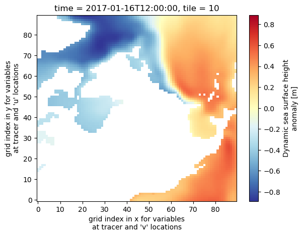
  uuid :

  9302811e-400c-11eb-b69e-0cc47a3f49c3

Now plot the SSH for Jan 2017 in tile 10 (Python numbering convention; 11 in Fortran/MATLAB numbering convention). Here we use the “RdYlBu” colormap, one of many built-in colormaps that the matplotlib package provides, or you can create your own. The “_r” at the end reverses the direction of the colormap, so red corresponds to the maximum values.

ds_SSH_s3.SSH.isel(time=0,tile=10).plot(cmap='RdYlBu_r')

<matplotlib.collections.QuadMesh at 0x7f1e08eff740>

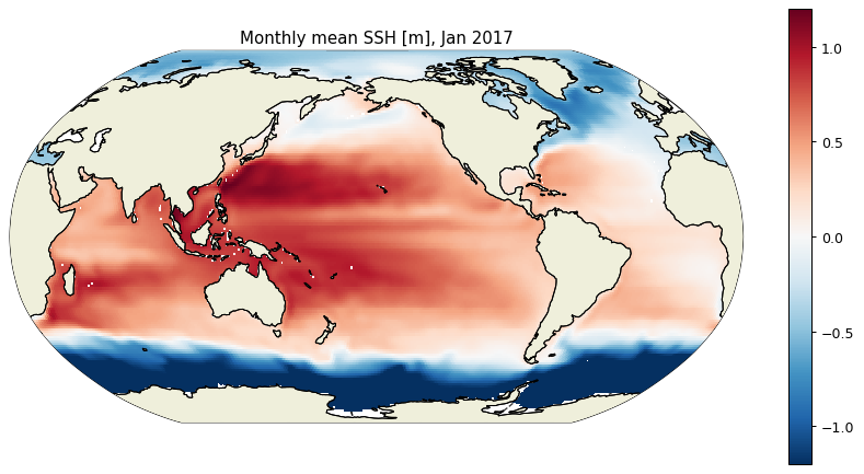
We can also use the ecco_v4_py package to plot a global map of Jan 2017 SSH, using the plot_proj_to_latlon_grid function which regrids from the native LLC grid to a lat/lon grid.

plt.figure(figsize=(12,6), dpi= 90)
ecco.plot_proj_to_latlon_grid(ds_SSH_s3.XC, ds_SSH_s3.YC, \
                              ds_SSH_s3.SSH.isel(time=0), \
                              user_lon_0=-160,\
                              projection_type='robin',\
                              plot_type='pcolormesh', \
                              cmap='RdBu_r',\
                              dx=1,dy=1,cmin=-1.2, cmax=1.2,show_colorbar=True)
plt.title('Monthly mean SSH [m], Jan 2017')
plt.show()

The ecco_podaac_access function

In-cloud direct access (mode = ‘s3_open’)

The ecco_podaac_to_xrdataset function that was previously used invokes ecco_podaac_access under the hood, and ecco_podaac_access can also be called directly. This can be useful if you want to obtain a list of file objects/paths or URLs that you can then process with your own code. Let’s use this function with mode = s3_open (all S3 modes only work from an AWS Cloud environment in region us-west-2).

curr_shortname = 'ECCO_L4_SSH_LLC0090GRID_MONTHLY_V4R4'
files_dict = ea.ecco_podaac_access(curr_shortname,\
                                    StartDate='2015-01',EndDate='2015-12',\
                                    mode='s3_open')

{'ShortName': 'ECCO_L4_SSH_LLC0090GRID_MONTHLY_V4R4', 'temporal': '2015-01-02,2015-12-31'}

Total number of matching granules: 12

files_dict[curr_shortname]

[<File-like object S3FileSystem, podaac-ops-cumulus-protected/ECCO_L4_SSH_LLC0090GRID_MONTHLY_V4R4/SEA_SURFACE_HEIGHT_mon_mean_2015-01_ECCO_V4r4_native_llc0090.nc>,
 <File-like object S3FileSystem, podaac-ops-cumulus-protected/ECCO_L4_SSH_LLC0090GRID_MONTHLY_V4R4/SEA_SURFACE_HEIGHT_mon_mean_2015-02_ECCO_V4r4_native_llc0090.nc>,
 <File-like object S3FileSystem, podaac-ops-cumulus-protected/ECCO_L4_SSH_LLC0090GRID_MONTHLY_V4R4/SEA_SURFACE_HEIGHT_mon_mean_2015-03_ECCO_V4r4_native_llc0090.nc>,
 <File-like object S3FileSystem, podaac-ops-cumulus-protected/ECCO_L4_SSH_LLC0090GRID_MONTHLY_V4R4/SEA_SURFACE_HEIGHT_mon_mean_2015-04_ECCO_V4r4_native_llc0090.nc>,
 <File-like object S3FileSystem, podaac-ops-cumulus-protected/ECCO_L4_SSH_LLC0090GRID_MONTHLY_V4R4/SEA_SURFACE_HEIGHT_mon_mean_2015-05_ECCO_V4r4_native_llc0090.nc>,
 <File-like object S3FileSystem, podaac-ops-cumulus-protected/ECCO_L4_SSH_LLC0090GRID_MONTHLY_V4R4/SEA_SURFACE_HEIGHT_mon_mean_2015-06_ECCO_V4r4_native_llc0090.nc>,
 <File-like object S3FileSystem, podaac-ops-cumulus-protected/ECCO_L4_SSH_LLC0090GRID_MONTHLY_V4R4/SEA_SURFACE_HEIGHT_mon_mean_2015-07_ECCO_V4r4_native_llc0090.nc>,
 <File-like object S3FileSystem, podaac-ops-cumulus-protected/ECCO_L4_SSH_LLC0090GRID_MONTHLY_V4R4/SEA_SURFACE_HEIGHT_mon_mean_2015-08_ECCO_V4r4_native_llc0090.nc>,
 <File-like object S3FileSystem, podaac-ops-cumulus-protected/ECCO_L4_SSH_LLC0090GRID_MONTHLY_V4R4/SEA_SURFACE_HEIGHT_mon_mean_2015-09_ECCO_V4r4_native_llc0090.nc>,
 <File-like object S3FileSystem, podaac-ops-cumulus-protected/ECCO_L4_SSH_LLC0090GRID_MONTHLY_V4R4/SEA_SURFACE_HEIGHT_mon_mean_2015-10_ECCO_V4r4_native_llc0090.nc>,
 <File-like object S3FileSystem, podaac-ops-cumulus-protected/ECCO_L4_SSH_LLC0090GRID_MONTHLY_V4R4/SEA_SURFACE_HEIGHT_mon_mean_2015-11_ECCO_V4r4_native_llc0090.nc>,
 <File-like object S3FileSystem, podaac-ops-cumulus-protected/ECCO_L4_SSH_LLC0090GRID_MONTHLY_V4R4/SEA_SURFACE_HEIGHT_mon_mean_2015-12_ECCO_V4r4_native_llc0090.nc>]

The output of ecco_podaac_access is in the form of a dictionary with ShortNames as keys. In this case, the value associated with this ShortName is a list of 12 file objects. These are files on S3 (AWS’s cloud storage system) that have been opened, which is a necessary step for the files’ data to be accessed. The list of open files can be passed directly to xarray.open_mfdataset.

ds_SSH_fromlist = xr.open_mfdataset(files_dict[curr_shortname],\
                                    compat='override',data_vars='minimal',coords='minimal',\
                                    parallel=True)

ds_SSH_fromlist

<xarray.Dataset> Size: 25MB
Dimensions:    (time: 12, tile: 13, j: 90, i: 90, i_g: 90, j_g: 90, nv: 2, nb: 4)
Coordinates: (12/13)
  * i          (i) int32 360B 0 1 2 3 4 5 6 7 8 9 ... 81 82 83 84 85 86 87 88 89
  * i_g        (i_g) int32 360B 0 1 2 3 4 5 6 7 8 ... 81 82 83 84 85 86 87 88 89
  * j          (j) int32 360B 0 1 2 3 4 5 6 7 8 9 ... 81 82 83 84 85 86 87 88 89
  * j_g        (j_g) int32 360B 0 1 2 3 4 5 6 7 8 ... 81 82 83 84 85 86 87 88 89
  * tile       (tile) int32 52B 0 1 2 3 4 5 6 7 8 9 10 11 12
  * time       (time) datetime64[ns] 96B 2015-01-16T12:00:00 ... 2015-12-16T1...
    ...         ...
    YC         (tile, j, i) float32 421kB dask.array<chunksize=(13, 90, 90), meta=np.ndarray>
    XG         (tile, j_g, i_g) float32 421kB dask.array<chunksize=(13, 90, 90), meta=np.ndarray>
    YG         (tile, j_g, i_g) float32 421kB dask.array<chunksize=(13, 90, 90), meta=np.ndarray>
    time_bnds  (time, nv) datetime64[ns] 192B dask.array<chunksize=(1, 2), meta=np.ndarray>
    XC_bnds    (tile, j, i, nb) float32 2MB dask.array<chunksize=(13, 90, 90, 4), meta=np.ndarray>
    YC_bnds    (tile, j, i, nb) float32 2MB dask.array<chunksize=(13, 90, 90, 4), meta=np.ndarray>
Dimensions without coordinates: nv, nb
Data variables:
    SSH        (time, tile, j, i) float32 5MB dask.array<chunksize=(1, 13, 90, 90), meta=np.ndarray>
    SSHIBC     (time, tile, j, i) float32 5MB dask.array<chunksize=(1, 13, 90, 90), meta=np.ndarray>
    SSHNOIBC   (time, tile, j, i) float32 5MB dask.array<chunksize=(1, 13, 90, 90), meta=np.ndarray>
    ETAN       (time, tile, j, i) float32 5MB dask.array<chunksize=(1, 13, 90, 90), meta=np.ndarray>
Attributes: (12/57)
    acknowledgement:              This research was carried out by the Jet Pr...
    author:                       Ian Fenty and Ou Wang
    cdm_data_type:                Grid
    comment:                      Fields provided on the curvilinear lat-lon-...
    Conventions:                  CF-1.8, ACDD-1.3
    coordinates_comment:          Note: the global 'coordinates' attribute de...
    ...                           ...
    time_coverage_duration:       P1M
    time_coverage_end:            2015-02-01T00:00:00
    time_coverage_resolution:     P1M
    time_coverage_start:          2015-01-01T00:00:00
    title:                        ECCO Sea Surface Height - Monthly Mean llc9...
    uuid:                         a4955186-400c-11eb-8c14-0cc47a3f49c3

xarray.Dataset

• Dimensions:
  • time: 12
  • tile: 13
  • j: 90
  • i: 90
  • i_g: 90
  • j_g: 90
  • nv: 2
  • nb: 4
• Coordinates: (13)
  • i
    (i)
    int32
    0 1 2 3 4 5 6 ... 84 85 86 87 88 89

    axis :

    X

    long_name :

    grid index in x for variables at tracer and 'v' locations

    swap_dim :

    XC

    comment :

    In the Arakawa C-grid system, tracer (e.g., THETA) and 'v' variables (e.g., VVEL) have the same x coordinate on the model grid.

    coverage_content_type :

    coordinate

    array([ 0,  1,  2,  3,  4,  5,  6,  7,  8,  9, 10, 11, 12, 13, 14, 15, 16, 17,
           18, 19, 20, 21, 22, 23, 24, 25, 26, 27, 28, 29, 30, 31, 32, 33, 34, 35,
           36, 37, 38, 39, 40, 41, 42, 43, 44, 45, 46, 47, 48, 49, 50, 51, 52, 53,
           54, 55, 56, 57, 58, 59, 60, 61, 62, 63, 64, 65, 66, 67, 68, 69, 70, 71,
           72, 73, 74, 75, 76, 77, 78, 79, 80, 81, 82, 83, 84, 85, 86, 87, 88, 89],
          dtype=int32)

  • i_g
    (i_g)
    int32
    0 1 2 3 4 5 6 ... 84 85 86 87 88 89

    axis :

    X

    long_name :

    grid index in x for variables at 'u' and 'g' locations

    c_grid_axis_shift :

    -0.5

    swap_dim :

    XG

    comment :

    In the Arakawa C-grid system, 'u' (e.g., UVEL) and 'g' variables (e.g., XG) have the same x coordinate on the model grid.

    coverage_content_type :

    coordinate

    array([ 0,  1,  2,  3,  4,  5,  6,  7,  8,  9, 10, 11, 12, 13, 14, 15, 16, 17,
           18, 19, 20, 21, 22, 23, 24, 25, 26, 27, 28, 29, 30, 31, 32, 33, 34, 35,
           36, 37, 38, 39, 40, 41, 42, 43, 44, 45, 46, 47, 48, 49, 50, 51, 52, 53,
           54, 55, 56, 57, 58, 59, 60, 61, 62, 63, 64, 65, 66, 67, 68, 69, 70, 71,
           72, 73, 74, 75, 76, 77, 78, 79, 80, 81, 82, 83, 84, 85, 86, 87, 88, 89],
          dtype=int32)

  • j
    (j)
    int32
    0 1 2 3 4 5 6 ... 84 85 86 87 88 89

    axis :

    Y

    long_name :

    grid index in y for variables at tracer and 'u' locations

    swap_dim :

    YC

    comment :

    In the Arakawa C-grid system, tracer (e.g., THETA) and 'u' variables (e.g., UVEL) have the same y coordinate on the model grid.

    coverage_content_type :

    coordinate

    array([ 0,  1,  2,  3,  4,  5,  6,  7,  8,  9, 10, 11, 12, 13, 14, 15, 16, 17,
           18, 19, 20, 21, 22, 23, 24, 25, 26, 27, 28, 29, 30, 31, 32, 33, 34, 35,
           36, 37, 38, 39, 40, 41, 42, 43, 44, 45, 46, 47, 48, 49, 50, 51, 52, 53,
           54, 55, 56, 57, 58, 59, 60, 61, 62, 63, 64, 65, 66, 67, 68, 69, 70, 71,
           72, 73, 74, 75, 76, 77, 78, 79, 80, 81, 82, 83, 84, 85, 86, 87, 88, 89],
          dtype=int32)

  • j_g
    (j_g)
    int32
    0 1 2 3 4 5 6 ... 84 85 86 87 88 89

    axis :

    Y

    long_name :

    grid index in y for variables at 'v' and 'g' locations

    c_grid_axis_shift :

    -0.5

    swap_dim :

    YG

    comment :

    In the Arakawa C-grid system, 'v' (e.g., VVEL) and 'g' variables (e.g., XG) have the same y coordinate.

    coverage_content_type :

    coordinate

    array([ 0,  1,  2,  3,  4,  5,  6,  7,  8,  9, 10, 11, 12, 13, 14, 15, 16, 17,
           18, 19, 20, 21, 22, 23, 24, 25, 26, 27, 28, 29, 30, 31, 32, 33, 34, 35,
           36, 37, 38, 39, 40, 41, 42, 43, 44, 45, 46, 47, 48, 49, 50, 51, 52, 53,
           54, 55, 56, 57, 58, 59, 60, 61, 62, 63, 64, 65, 66, 67, 68, 69, 70, 71,
           72, 73, 74, 75, 76, 77, 78, 79, 80, 81, 82, 83, 84, 85, 86, 87, 88, 89],
          dtype=int32)

  • tile
    (tile)
    int32
    0 1 2 3 4 5 6 7 8 9 10 11 12

    long_name :

    lat-lon-cap tile index

    comment :

    The ECCO V4 horizontal model grid is divided into 13 tiles of 90x90 cells for convenience.

    coverage_content_type :

    coordinate

    array([ 0,  1,  2,  3,  4,  5,  6,  7,  8,  9, 10, 11, 12], dtype=int32)

  • time
    (time)
    datetime64[ns]
    2015-01-16T12:00:00 ... 2015-12-...

    long_name :

    center time of averaging period

    axis :

    T

    bounds :

    time_bnds

    coverage_content_type :

    coordinate

    standard_name :

    time

    array(['2015-01-16T12:00:00.000000000', '2015-02-15T00:00:00.000000000',
           '2015-03-16T12:00:00.000000000', '2015-04-16T00:00:00.000000000',
           '2015-05-16T12:00:00.000000000', '2015-06-16T00:00:00.000000000',
           '2015-07-16T12:00:00.000000000', '2015-08-16T12:00:00.000000000',
           '2015-09-16T00:00:00.000000000', '2015-10-16T12:00:00.000000000',
           '2015-11-16T00:00:00.000000000', '2015-12-16T12:00:00.000000000'],
          dtype='datetime64[ns]')

  • XC
    (tile, j, i)
    float32
    dask.array<chunksize=(13, 90, 90), meta=np.ndarray>

    long_name :

    longitude of tracer grid cell center

    units :

    degrees_east

    coordinate :

    YC XC

    bounds :

    XC_bnds

    comment :

    nonuniform grid spacing

    coverage_content_type :

    coordinate

    standard_name :

    longitude

    Array Chunk Bytes 411.33 kiB 411.33 kiB Shape (13, 90, 90) (13, 90, 90) Dask graph 1 chunks in 2 graph layers Data type float32 numpy.ndarray

  • YC
    (tile, j, i)
    float32
    dask.array<chunksize=(13, 90, 90), meta=np.ndarray>

    long_name :

    latitude of tracer grid cell center

    units :

    degrees_north

    coordinate :

    YC XC

    bounds :

    YC_bnds

    comment :

    nonuniform grid spacing

    coverage_content_type :

    coordinate

    standard_name :

    latitude

    Array Chunk Bytes 411.33 kiB 411.33 kiB Shape (13, 90, 90) (13, 90, 90) Dask graph 1 chunks in 2 graph layers Data type float32 numpy.ndarray

  • XG
    (tile, j_g, i_g)
    float32
    dask.array<chunksize=(13, 90, 90), meta=np.ndarray>

    long_name :

    longitude of 'southwest' corner of tracer grid cell

    units :

    degrees_east

    coordinate :

    YG XG

    comment :

    Nonuniform grid spacing. Note: 'southwest' does not correspond to geographic orientation but is used for convenience to describe the computational grid. See MITgcm dcoumentation for details.

    coverage_content_type :

    coordinate

    standard_name :

    longitude

    Array Chunk Bytes 411.33 kiB 411.33 kiB Shape (13, 90, 90) (13, 90, 90) Dask graph 1 chunks in 2 graph layers Data type float32 numpy.ndarray

  • YG
    (tile, j_g, i_g)
    float32
    dask.array<chunksize=(13, 90, 90), meta=np.ndarray>

    long_name :

    latitude of 'southwest' corner of tracer grid cell

    units :

    degrees_north

    coordinate :

    YG XG

    comment :

    Nonuniform grid spacing. Note: 'southwest' does not correspond to geographic orientation but is used for convenience to describe the computational grid. See MITgcm dcoumentation for details.

    coverage_content_type :

    coordinate

    standard_name :

    latitude

    Array Chunk Bytes 411.33 kiB 411.33 kiB Shape (13, 90, 90) (13, 90, 90) Dask graph 1 chunks in 2 graph layers Data type float32 numpy.ndarray

  • time_bnds
    (time, nv)
    datetime64[ns]
    dask.array<chunksize=(1, 2), meta=np.ndarray>

    comment :

    Start and end times of averaging period.

    coverage_content_type :

    coordinate

    long_name :

    time bounds of averaging period

    Array Chunk Bytes 192 B 16 B Shape (12, 2) (1, 2) Dask graph 12 chunks in 25 graph layers Data type datetime64[ns] numpy.ndarray

  • XC_bnds
    (tile, j, i, nb)
    float32
    dask.array<chunksize=(13, 90, 90, 4), meta=np.ndarray>

    comment :

    Bounds array follows CF conventions. XC_bnds[i,j,0] = 'southwest' corner (j-1, i-1), XC_bnds[i,j,1] = 'southeast' corner (j-1, i+1), XC_bnds[i,j,2] = 'northeast' corner (j+1, i+1), XC_bnds[i,j,3] = 'northwest' corner (j+1, i-1). Note: 'southwest', 'southeast', northwest', and 'northeast' do not correspond to geographic orientation but are used for convenience to describe the computational grid. See MITgcm dcoumentation for details.

    coverage_content_type :

    coordinate

    long_name :

    longitudes of tracer grid cell corners

    Array Chunk Bytes 1.61 MiB 1.61 MiB Shape (13, 90, 90, 4) (13, 90, 90, 4) Dask graph 1 chunks in 2 graph layers Data type float32 numpy.ndarray

  • YC_bnds
    (tile, j, i, nb)
    float32
    dask.array<chunksize=(13, 90, 90, 4), meta=np.ndarray>

    comment :

    Bounds array follows CF conventions. YC_bnds[i,j,0] = 'southwest' corner (j-1, i-1), YC_bnds[i,j,1] = 'southeast' corner (j-1, i+1), YC_bnds[i,j,2] = 'northeast' corner (j+1, i+1), YC_bnds[i,j,3] = 'northwest' corner (j+1, i-1). Note: 'southwest', 'southeast', northwest', and 'northeast' do not correspond to geographic orientation but are used for convenience to describe the computational grid. See MITgcm dcoumentation for details.

    coverage_content_type :

    coordinate

    long_name :

    latitudes of tracer grid cell corners

    Array Chunk Bytes 1.61 MiB 1.61 MiB Shape (13, 90, 90, 4) (13, 90, 90, 4) Dask graph 1 chunks in 2 graph layers Data type float32 numpy.ndarray

• Data variables: (4)
  • SSH
    (time, tile, j, i)
    float32
    dask.array<chunksize=(1, 13, 90, 90), meta=np.ndarray>

    long_name :

    Dynamic sea surface height anomaly

    units :

    m

    coverage_content_type :

    modelResult

    standard_name :

    sea_surface_height_above_geoid

    comment :

    Dynamic sea surface height anomaly above the geoid, suitable for comparisons with altimetry sea surface height data products that apply the inverse barometer (IB) correction. Note: SSH is calculated by correcting model sea level anomaly ETAN for three effects: a) global mean steric sea level changes related to density changes in the Boussinesq volume-conserving model (Greatbatch correction, see sterGloH), b) the inverted barometer (IB) effect (see SSHIBC) and c) sea level displacement due to sea-ice and snow pressure loading (see sIceLoad). SSH can be compared with the similarly-named SSH variable in previous ECCO products that did not include atmospheric pressure loading (e.g., Version 4 Release 3). Use SSHNOIBC for comparisons with altimetry data products that do NOT apply the IB correction.

    valid_min :

    -1.8805772066116333

    valid_max :

    1.4207719564437866

    Array Chunk Bytes 4.82 MiB 411.33 kiB Shape (12, 13, 90, 90) (1, 13, 90, 90) Dask graph 12 chunks in 25 graph layers Data type float32 numpy.ndarray

  • SSHIBC
    (time, tile, j, i)
    float32
    dask.array<chunksize=(1, 13, 90, 90), meta=np.ndarray>

    long_name :

    The inverted barometer (IB) correction to sea surface height due to atmospheric pressure loading

    units :

    m

    coverage_content_type :

    modelResult

    comment :

    Not an SSH itself, but a correction to model sea level anomaly (ETAN) required to account for the static part of sea surface displacement by atmosphere pressure loading: SSH = SSHNOIBC - SSHIBC. Note: Use SSH for model-data comparisons with altimetry data products that DO apply the IB correction and SSHNOIBC for comparisons with altimetry data products that do NOT apply the IB correction.

    valid_min :

    -0.30144819617271423

    valid_max :

    0.5248842239379883

    Array Chunk Bytes 4.82 MiB 411.33 kiB Shape (12, 13, 90, 90) (1, 13, 90, 90) Dask graph 12 chunks in 25 graph layers Data type float32 numpy.ndarray

  • SSHNOIBC
    (time, tile, j, i)
    float32
    dask.array<chunksize=(1, 13, 90, 90), meta=np.ndarray>

    long_name :

    Sea surface height anomaly without the inverted barometer (IB) correction

    units :

    m

    coverage_content_type :

    modelResult

    comment :

    Sea surface height anomaly above the geoid without the inverse barometer (IB) correction, suitable for comparisons with altimetry sea surface height data products that do NOT apply the inverse barometer (IB) correction. Note: SSHNOIBC is calculated by correcting model sea level anomaly ETAN for two effects: a) global mean steric sea level changes related to density changes in the Boussinesq volume-conserving model (Greatbatch correction, see sterGloH), b) sea level displacement due to sea-ice and snow pressure loading (see sIceLoad). In ECCO Version 4 Release 4 the model is forced with atmospheric pressure loading. SSHNOIBC does not correct for the static part of the effect of atmosphere pressure loading on sea surface height (the so-called inverse barometer (IB) correction). Use SSH for comparisons with altimetry data products that DO apply the IB correction.

    valid_min :

    -1.6654272079467773

    valid_max :

    1.4550364017486572

    Array Chunk Bytes 4.82 MiB 411.33 kiB Shape (12, 13, 90, 90) (1, 13, 90, 90) Dask graph 12 chunks in 25 graph layers Data type float32 numpy.ndarray

  • ETAN
    (time, tile, j, i)
    float32
    dask.array<chunksize=(1, 13, 90, 90), meta=np.ndarray>

    long_name :

    Model sea level anomaly

    units :

    m

    coverage_content_type :

    modelResult

    comment :

    Model sea level anomaly WITHOUT corrections for global mean density (steric) changes, inverted barometer effect, or volume displacement due to submerged sea-ice and snow . Note: ETAN should NOT be used for comparisons with altimetry data products because ETAN is NOT corrected for (a) global mean steric sea level changes related to density changes in the Boussinesq volume-conserving model (Greatbatch correction, see sterGloH) nor (b) sea level displacement due to submerged sea-ice and snow (see sIceLoad). These corrections ARE made for the variables SSH and SSHNOIBC.

    valid_min :

    -8.304216384887695

    valid_max :

    1.460192084312439

    Array Chunk Bytes 4.82 MiB 411.33 kiB Shape (12, 13, 90, 90) (1, 13, 90, 90) Dask graph 12 chunks in 25 graph layers Data type float32 numpy.ndarray

• Indexes: (6)
  • i
    PandasIndex

    PandasIndex(Index([ 0,  1,  2,  3,  4,  5,  6,  7,  8,  9, 10, 11, 12, 13, 14, 15, 16, 17,
           18, 19, 20, 21, 22, 23, 24, 25, 26, 27, 28, 29, 30, 31, 32, 33, 34, 35,
           36, 37, 38, 39, 40, 41, 42, 43, 44, 45, 46, 47, 48, 49, 50, 51, 52, 53,
           54, 55, 56, 57, 58, 59, 60, 61, 62, 63, 64, 65, 66, 67, 68, 69, 70, 71,
           72, 73, 74, 75, 76, 77, 78, 79, 80, 81, 82, 83, 84, 85, 86, 87, 88, 89],
          dtype='int32', name='i'))

  • i_g
    PandasIndex

    PandasIndex(Index([ 0,  1,  2,  3,  4,  5,  6,  7,  8,  9, 10, 11, 12, 13, 14, 15, 16, 17,
           18, 19, 20, 21, 22, 23, 24, 25, 26, 27, 28, 29, 30, 31, 32, 33, 34, 35,
           36, 37, 38, 39, 40, 41, 42, 43, 44, 45, 46, 47, 48, 49, 50, 51, 52, 53,
           54, 55, 56, 57, 58, 59, 60, 61, 62, 63, 64, 65, 66, 67, 68, 69, 70, 71,
           72, 73, 74, 75, 76, 77, 78, 79, 80, 81, 82, 83, 84, 85, 86, 87, 88, 89],
          dtype='int32', name='i_g'))

  • j
    PandasIndex

    PandasIndex(Index([ 0,  1,  2,  3,  4,  5,  6,  7,  8,  9, 10, 11, 12, 13, 14, 15, 16, 17,
           18, 19, 20, 21, 22, 23, 24, 25, 26, 27, 28, 29, 30, 31, 32, 33, 34, 35,
           36, 37, 38, 39, 40, 41, 42, 43, 44, 45, 46, 47, 48, 49, 50, 51, 52, 53,
           54, 55, 56, 57, 58, 59, 60, 61, 62, 63, 64, 65, 66, 67, 68, 69, 70, 71,
           72, 73, 74, 75, 76, 77, 78, 79, 80, 81, 82, 83, 84, 85, 86, 87, 88, 89],
          dtype='int32', name='j'))

  • j_g
    PandasIndex

    PandasIndex(Index([ 0,  1,  2,  3,  4,  5,  6,  7,  8,  9, 10, 11, 12, 13, 14, 15, 16, 17,
           18, 19, 20, 21, 22, 23, 24, 25, 26, 27, 28, 29, 30, 31, 32, 33, 34, 35,
           36, 37, 38, 39, 40, 41, 42, 43, 44, 45, 46, 47, 48, 49, 50, 51, 52, 53,
           54, 55, 56, 57, 58, 59, 60, 61, 62, 63, 64, 65, 66, 67, 68, 69, 70, 71,
           72, 73, 74, 75, 76, 77, 78, 79, 80, 81, 82, 83, 84, 85, 86, 87, 88, 89],
          dtype='int32', name='j_g'))

  • tile
    PandasIndex

    PandasIndex(Index([0, 1, 2, 3, 4, 5, 6, 7, 8, 9, 10, 11, 12], dtype='int32', name='tile'))

  • time
    PandasIndex

    PandasIndex(DatetimeIndex(['2015-01-16 12:00:00', '2015-02-15 00:00:00',
                   '2015-03-16 12:00:00', '2015-04-16 00:00:00',
                   '2015-05-16 12:00:00', '2015-06-16 00:00:00',
                   '2015-07-16 12:00:00', '2015-08-16 12:00:00',
                   '2015-09-16 00:00:00', '2015-10-16 12:00:00',
                   '2015-11-16 00:00:00', '2015-12-16 12:00:00'],
                  dtype='datetime64[ns]', name='time', freq=None))

• Attributes: (57)

  acknowledgement :

  This research was carried out by the Jet Propulsion Laboratory, managed by the California Institute of Technology under a contract with the National Aeronautics and Space Administration.

  author :

  Ian Fenty and Ou Wang

  cdm_data_type :

  Grid

  comment :

  Fields provided on the curvilinear lat-lon-cap 90 (llc90) native grid used in the ECCO model. SSH (dynamic sea surface height) = SSHNOIBC (dynamic sea surface without the inverse barometer correction) - SSHIBC (inverse barometer correction). The inverted barometer correction accounts for variations in sea surface height due to atmospheric pressure variations. Note: ETAN is model sea level anomaly and should not be compared with satellite altimetery products, see SSH and ETAN for more details.

  Conventions :

  CF-1.8, ACDD-1.3

  coordinates_comment :

  Note: the global 'coordinates' attribute describes auxillary coordinates.

  creator_email :

  ecco-group@mit.edu

  creator_institution :

  NASA Jet Propulsion Laboratory (JPL)

  creator_name :

  ECCO Consortium

  creator_type :

  group

  creator_url :

  https://ecco-group.org

  date_created :

  2020-12-16T18:07:40

  date_issued :

  2020-12-16T18:07:40

  date_metadata_modified :

  2021-03-15T21:56:49

  date_modified :

  2021-03-15T21:56:49

  geospatial_bounds_crs :

  EPSG:4326

  geospatial_lat_max :

  90.0

  geospatial_lat_min :

  -90.0

  geospatial_lat_resolution :

  variable

  geospatial_lat_units :

  degrees_north

  geospatial_lon_max :

  180.0

  geospatial_lon_min :

  -180.0

  geospatial_lon_resolution :

  variable

  geospatial_lon_units :

  degrees_east

  history :

  Inaugural release of an ECCO Central Estimate solution to PO.DAAC

  id :

  10.5067/ECL5M-SSH44

  institution :

  NASA Jet Propulsion Laboratory (JPL)

  instrument_vocabulary :

  GCMD instrument keywords

  keywords :

  EARTH SCIENCE SERVICES > MODELS > EARTH SCIENCE REANALYSES/ASSIMILATION MODELS, EARTH SCIENCE > OCEANS > SEA SURFACE TOPOGRAPHY > SEA SURFACE HEIGHT

  keywords_vocabulary :

  NASA Global Change Master Directory (GCMD) Science Keywords

  license :

  Public Domain

  metadata_link :

  https://cmr.earthdata.nasa.gov/search/collections.umm_json?ShortName=ECCO_L4_SSH_LLC0090GRID_MONTHLY_V4R4

  naming_authority :

  gov.nasa.jpl

  platform :

  ERS-1/2, TOPEX/Poseidon, Geosat Follow-On (GFO), ENVISAT, Jason-1, Jason-2, CryoSat-2, SARAL/AltiKa, Jason-3, AVHRR, Aquarius, SSM/I, SSMIS, GRACE, DTU17MDT, Argo, WOCE, GO-SHIP, MEOP, Ice Tethered Profilers (ITP)

  platform_vocabulary :

  GCMD platform keywords

  processing_level :

  L4

  product_name :

  SEA_SURFACE_HEIGHT_mon_mean_2015-01_ECCO_V4r4_native_llc0090.nc

  product_time_coverage_end :

  2018-01-01T00:00:00

  product_time_coverage_start :

  1992-01-01T12:00:00

  product_version :

  Version 4, Release 4

  program :

  NASA Physical Oceanography, Cryosphere, Modeling, Analysis, and Prediction (MAP)

  project :

  Estimating the Circulation and Climate of the Ocean (ECCO)

  publisher_email :

  podaac@podaac.jpl.nasa.gov

  publisher_institution :

  PO.DAAC

  publisher_name :

  Physical Oceanography Distributed Active Archive Center (PO.DAAC)

  publisher_type :

  institution

  publisher_url :

  https://podaac.jpl.nasa.gov

  references :

  ECCO Consortium, Fukumori, I., Wang, O., Fenty, I., Forget, G., Heimbach, P., & Ponte, R. M. 2020. Synopsis of the ECCO Central Production Global Ocean and Sea-Ice State Estimate (Version 4 Release 4). doi:10.5281/zenodo.3765928

  source :

  The ECCO V4r4 state estimate was produced by fitting a free-running solution of the MITgcm (checkpoint 66g) to satellite and in situ observational data in a least squares sense using the adjoint method

  standard_name_vocabulary :

  NetCDF Climate and Forecast (CF) Metadata Convention

  summary :

  This dataset provides monthly-averaged dynamic sea surface height and model sea level anomaly on the lat-lon-cap 90 (llc90) native model grid from the ECCO Version 4 Release 4 (V4r4) ocean and sea-ice state estimate. Estimating the Circulation and Climate of the Ocean (ECCO) state estimates are dynamically and kinematically-consistent reconstructions of the three-dimensional, time-evolving ocean, sea-ice, and surface atmospheric states. ECCO V4r4 is a free-running solution of a global, nominally 1-degree configuration of the MIT general circulation model (MITgcm) that has been fit to observations in a least-squares sense. Observational data constraints used in V4r4 include sea surface height (SSH) from satellite altimeters [ERS-1/2, TOPEX/Poseidon, GFO, ENVISAT, Jason-1,2,3, CryoSat-2, and SARAL/AltiKa]; sea surface temperature (SST) from satellite radiometers [AVHRR], sea surface salinity (SSS) from the Aquarius satellite radiometer/scatterometer, ocean bottom pressure (OBP) from the GRACE satellite gravimeter; sea-ice concentration from satellite radiometers [SSM/I and SSMIS], and in-situ ocean temperature and salinity measured with conductivity-temperature-depth (CTD) sensors and expendable bathythermographs (XBTs) from several programs [e.g., WOCE, GO-SHIP, Argo, and others] and platforms [e.g., research vessels, gliders, moorings, ice-tethered profilers, and instrumented pinnipeds]. V4r4 covers the period 1992-01-01T12:00:00 to 2018-01-01T00:00:00.

  time_coverage_duration :

  P1M

  time_coverage_end :

  2015-02-01T00:00:00

  time_coverage_resolution :

  P1M

  time_coverage_start :

  2015-01-01T00:00:00

  title :

  ECCO Sea Surface Height - Monthly Mean llc90 Grid (Version 4 Release 4)

  uuid :

  a4955186-400c-11eb-8c14-0cc47a3f49c3