Accessing ECCOv4 release 5 output in the AWS Cloud

Introduction

SST comparison: v4r4 vs. v4r5

Momentum budget terms in v4r5

Introduction

In addition to accessing the ECCOv4r4 Central Estimate output released on PO.DAAC, ecco_access functions can also retrieve output from the newer release 5 (ECCOv4r5). Unlike v4r4, for which many fields can be accessed at monthly/daily/snapshot time resolutions and native/latlon grid configurations, only the v4r5 monthly mean native grid outputs are currently accessible, and ecco_access can only retrieve them within the AWS Cloud. However, a number of fields were archived in v4r5 that were not archived in v4r4, including the terms of momentum and sea-ice budgets.

SST comparison: v4r4 vs. v4r5

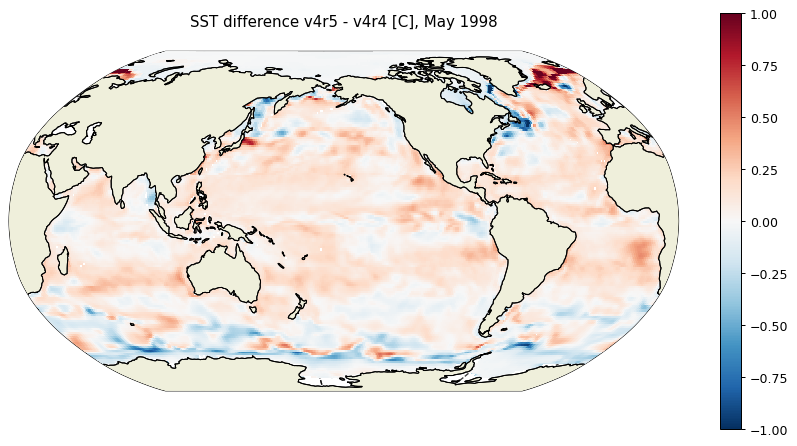
First let’s consider a field that is archived in both releases: potential temperature in the top layer, or SST. Accessing the monthly mean potential temperature for 1998 from v4r4 (and assuming we don’t know the ShortName already):

import xarray as xr
import matplotlib.pyplot as plt
from os.path import join,expanduser

import ecco_v4_py as ecco
import ecco_access as ea

# identify user's home directory
user_home_dir = expanduser('~')

Note: If using s3_open_fsspec mode, you will need access to json files that are hosted on the s3://ecco-model-granules/ bucket, a “requester pays” bucket. This means that the entity requesting the data (i.e., you) would pay the data transfer fees. However, no need to get alarmed! When transferring data within the same AWS region as the bucket, the requester does not have to pay any data transfer fees. If your AWS EC2 instance is set up in the same region us-west-2 (Oregon) as the ecco-model-granules bucket, there will be no cost associated with the data transfer.

When accessing data from the ecco-model-granules bucket, a prompt appears by default to remind the user that the data access is “requester pays”. This prompt can be suppressed by setting prompt_request_payer=False.

# open v4r4 monthly v4r4 temperature fields for 1998, using s3_open_fsspec mode
ds_T_v4r4 = ea.ecco_podaac_to_xrdataset('temperature',\
                                            version='v4r4',grid='native',time_res='monthly',\
                                            StartDate='1998-01',EndDate='1998-12',\
                                            mode='s3_open_fsspec',\
                                            prompt_request_payer=False)

ShortName Options for query "temperature":
                  Variable Name     Description (units)

Option 1: ECCO_L4_ATM_STATE_LLC0090GRID_MONTHLY_V4R4    *native grid,monthly means*
                  EXFatemp          Atmosphere surface (2 m) air temperature (degK)
                  EXFaqh            Atmosphere surface (2 m) specific humidity (kg/kg)
                  EXFuwind          Wind speed at 10m in the model +x direction (m/s)
                  EXFvwind          Wind speed at 10m in the model +y direction (m/s)
                  EXFwspee          Wind speed (m/s)
                  EXFpress          Atmosphere surface pressure (N/m^2)

Option 2: ECCO_L4_HEAT_FLUX_LLC0090GRID_MONTHLY_V4R4    *native grid,monthly means*
                  EXFhl             Open ocean air-sea latent heat flux (W/m^2)
                  EXFhs             Open ocean air-sea sensible heat flux (W/m^2)
                  EXFlwdn           Downward longwave radiative flux (W/m^2)
                  EXFswdn           Downwelling shortwave radiative flux (W/m^2)
                  EXFqnet           Open ocean net air-sea heat flux (W/m^2)
                  oceQnet           Net heat flux into the ocean surface (W/m^2)
                  SIatmQnt          Net upward heat flux to the atmosphere (W/m^2)
                  TFLUX             Rate of change of ocean heat content per m^2
                                    accounting for mass (e.g. freshwater) fluxes
                                    (W/m^2)
                  EXFswnet          Open ocean net shortwave radiative flux (W/m^2)
                  EXFlwnet          Net open ocean longwave radiative flux (W/m^2)
                  oceQsw            Net shortwave radiative flux across the ocean
                                    surface (W/m^2)
                  SIaaflux          Conservative ocean and sea-ice advective heat flux
                                    adjustment, associated with temperature difference
                                    between sea surface temperature and sea-ice,
                                    excluding latent heat of fusion (W/m^2)

Option 3: ECCO_L4_MIXED_LAYER_DEPTH_LLC0090GRID_MONTHLY_V4R4    *native grid,monthly means*
                  MXLDEPTH          Mixed-layer depth diagnosed using the temperature
                                    difference criterion of Kara et al., 2000 (m)

Option 4: ECCO_L4_TEMP_SALINITY_LLC0090GRID_MONTHLY_V4R4    *native grid,monthly means*
                  THETA             Potential temperature, i.e., temperature of water
                                    parcel at sea level pressure (degC)
                  SALT              Salinity (1e-3, or parts per thousand)

Option 5: ECCO_L4_OCEAN_3D_TEMPERATURE_FLUX_LLC0090GRID_MONTHLY_V4R4    *native grid,monthly means*
                  ADVx_TH           Lateral advective flux of potential temperature in
                                    the model +x direction (degC m^3/s)
                  ADVy_TH           Lateral advective flux of potential temperature in
                                    the model +y direction (degC m^3/s)
                  ADVr_TH           Vertical advective flux of potential temperature
                                    (degC m^3/s)
                  DFxE_TH           Lateral diffusive flux of potential temperature in
                                    the model +x direction (degC m^3/s)
                  DFyE_TH           Lateral diffusive flux of potential temperature in
                                    the model +y direction (degC m^3/s)
                  DFrE_TH           Vertical diffusive flux of potential temperature,
                                    explicit term (degC m^3/s)
                  DFrI_TH           Vertical diffusive flux of potential temperature,
                                    implicit term (degC m^3/s)

Please select option [1-5]:  4

Using dataset with ShortName: ECCO_L4_TEMP_SALINITY_LLC0090GRID_MONTHLY_V4R4

Select option 4 (the dataset that contains variables THETA and SALT), and the requested output is included in the xarray dataset ds_T_v4r4. Here is the contents of that dataset:

ds_T_v4r4

<xarray.Dataset> Size: 510MB
Dimensions:    (time: 12, k: 50, tile: 13, j: 90, i: 90, nb: 4, j_g: 90,
                i_g: 90, nv: 2, k_l: 50, k_p1: 51, k_u: 50)
Coordinates: (12/22)
  * time       (time) datetime64[ns] 96B 1998-01-16T12:00:00 ... 1998-12-16T1...
    XC         (tile, j, i) float32 421kB dask.array<chunksize=(13, 90, 90), meta=np.ndarray>
    XC_bnds    (tile, j, i, nb) float32 2MB dask.array<chunksize=(13, 90, 90, 4), meta=np.ndarray>
    XG         (tile, j_g, i_g) float32 421kB dask.array<chunksize=(13, 90, 90), meta=np.ndarray>
    YC         (tile, j, i) float32 421kB dask.array<chunksize=(13, 90, 90), meta=np.ndarray>
    YC_bnds    (tile, j, i, nb) float32 2MB dask.array<chunksize=(13, 90, 90, 4), meta=np.ndarray>
    ...         ...
  * k          (k) int32 200B 0 1 2 3 4 5 6 7 8 9 ... 41 42 43 44 45 46 47 48 49
  * k_l        (k_l) int32 200B 0 1 2 3 4 5 6 7 8 ... 41 42 43 44 45 46 47 48 49
  * k_p1       (k_p1) int32 204B 0 1 2 3 4 5 6 7 8 ... 43 44 45 46 47 48 49 50
  * k_u        (k_u) int32 200B 0 1 2 3 4 5 6 7 8 ... 41 42 43 44 45 46 47 48 49
  * tile       (tile) int32 52B 0 1 2 3 4 5 6 7 8 9 10 11 12
    time_bnds  (time, nv) datetime64[ns] 192B dask.array<chunksize=(12, 2), meta=np.ndarray>
Dimensions without coordinates: nb, nv
Data variables:
    SALT       (time, k, tile, j, i) float32 253MB dask.array<chunksize=(6, 50, 13, 90, 90), meta=np.ndarray>
    THETA      (time, k, tile, j, i) float32 253MB dask.array<chunksize=(6, 50, 13, 90, 90), meta=np.ndarray>
Attributes: (12/62)
    Conventions:                     CF-1.8, ACDD-1.3
    acknowledgement:                 This research was carried out by the Jet...
    author:                          Ian Fenty and Ou Wang
    cdm_data_type:                   Grid
    comment:                         Fields provided on the curvilinear lat-l...
    coordinates_comment:             Note: the global 'coordinates' attribute...
    ...                              ...
    time_coverage_duration:          P1M
    time_coverage_end:               1992-02-01T00:00:00
    time_coverage_resolution:        P1M
    time_coverage_start:             1992-01-01T12:00:00
    title:                           ECCO Ocean Temperature and Salinity - Mo...
    uuid:                            f07693e6-4181-11eb-beb3-0cc47a3f44ff

xarray.Dataset

• Dimensions:
  • time: 12
  • k: 50
  • tile: 13
  • j: 90
  • i: 90
  • nb: 4
  • j_g: 90
  • i_g: 90
  • nv: 2
  • k_l: 50
  • k_p1: 51
  • k_u: 50
• Coordinates: (22)
  • time
    (time)
    datetime64[ns]
    1998-01-16T12:00:00 ... 1998-12-...

    axis :

    T

    bounds :

    time_bnds

    coverage_content_type :

    coordinate

    long_name :

    center time of averaging period

    standard_name :

    time

    array(['1998-01-16T12:00:00.000000000', '1998-02-15T00:00:00.000000000',
           '1998-03-16T12:00:00.000000000', '1998-04-16T00:00:00.000000000',
           '1998-05-16T12:00:00.000000000', '1998-06-16T00:00:00.000000000',
           '1998-07-16T12:00:00.000000000', '1998-08-16T12:00:00.000000000',
           '1998-09-16T00:00:00.000000000', '1998-10-16T12:00:00.000000000',
           '1998-11-16T00:00:00.000000000', '1998-12-16T12:00:00.000000000'],
          dtype='datetime64[ns]')

  • XC
    (tile, j, i)
    float32
    dask.array<chunksize=(13, 90, 90), meta=np.ndarray>

    bounds :

    XC_bnds

    comment :

    nonuniform grid spacing

    coordinate :

    YC XC

    coverage_content_type :

    coordinate

    long_name :

    longitude of tracer grid cell center

    standard_name :

    longitude

    units :

    degrees_east

    Array Chunk Bytes 411.33 kiB 411.33 kiB Shape (13, 90, 90) (13, 90, 90) Dask graph 1 chunks in 2 graph layers Data type float32 numpy.ndarray

  • XC_bnds
    (tile, j, i, nb)
    float32
    dask.array<chunksize=(13, 90, 90, 4), meta=np.ndarray>

    comment :

    Bounds array follows CF conventions. XC_bnds[i,j,0] = 'southwest' corner (j-1, i-1), XC_bnds[i,j,1] = 'southeast' corner (j-1, i+1), XC_bnds[i,j,2] = 'northeast' corner (j+1, i+1), XC_bnds[i,j,3] = 'northwest' corner (j+1, i-1). Note: 'southwest', 'southeast', northwest', and 'northeast' do not correspond to geographic orientation but are used for convenience to describe the computational grid. See MITgcm dcoumentation for details.

    coverage_content_type :

    coordinate

    long_name :

    longitudes of tracer grid cell corners

    Array Chunk Bytes 1.61 MiB 1.61 MiB Shape (13, 90, 90, 4) (13, 90, 90, 4) Dask graph 1 chunks in 2 graph layers Data type float32 numpy.ndarray

  • XG
    (tile, j_g, i_g)
    float32
    dask.array<chunksize=(13, 90, 90), meta=np.ndarray>

    comment :

    Nonuniform grid spacing. Note: 'southwest' does not correspond to geographic orientation but is used for convenience to describe the computational grid. See MITgcm dcoumentation for details.

    coordinate :

    YG XG

    coverage_content_type :

    coordinate

    long_name :

    longitude of 'southwest' corner of tracer grid cell

    standard_name :

    longitude

    units :

    degrees_east

    Array Chunk Bytes 411.33 kiB 411.33 kiB Shape (13, 90, 90) (13, 90, 90) Dask graph 1 chunks in 2 graph layers Data type float32 numpy.ndarray

  • YC
    (tile, j, i)
    float32
    dask.array<chunksize=(13, 90, 90), meta=np.ndarray>

    bounds :

    YC_bnds

    comment :

    nonuniform grid spacing

    coordinate :

    YC XC

    coverage_content_type :

    coordinate

    long_name :

    latitude of tracer grid cell center

    standard_name :

    latitude

    units :

    degrees_north

    Array Chunk Bytes 411.33 kiB 411.33 kiB Shape (13, 90, 90) (13, 90, 90) Dask graph 1 chunks in 2 graph layers Data type float32 numpy.ndarray

  • YC_bnds
    (tile, j, i, nb)
    float32
    dask.array<chunksize=(13, 90, 90, 4), meta=np.ndarray>

    comment :

    Bounds array follows CF conventions. YC_bnds[i,j,0] = 'southwest' corner (j-1, i-1), YC_bnds[i,j,1] = 'southeast' corner (j-1, i+1), YC_bnds[i,j,2] = 'northeast' corner (j+1, i+1), YC_bnds[i,j,3] = 'northwest' corner (j+1, i-1). Note: 'southwest', 'southeast', northwest', and 'northeast' do not correspond to geographic orientation but are used for convenience to describe the computational grid. See MITgcm dcoumentation for details.

    coverage_content_type :

    coordinate

    long_name :

    latitudes of tracer grid cell corners

    Array Chunk Bytes 1.61 MiB 1.61 MiB Shape (13, 90, 90, 4) (13, 90, 90, 4) Dask graph 1 chunks in 2 graph layers Data type float32 numpy.ndarray

  • YG
    (tile, j_g, i_g)
    float32
    dask.array<chunksize=(13, 90, 90), meta=np.ndarray>

    comment :

    Nonuniform grid spacing. Note: 'southwest' does not correspond to geographic orientation but is used for convenience to describe the computational grid. See MITgcm dcoumentation for details.

    coordinate :

    YG XG

    coverage_content_type :

    coordinate

    long_name :

    latitude of 'southwest' corner of tracer grid cell

    standard_name :

    latitude

    units :

    degrees_north

    Array Chunk Bytes 411.33 kiB 411.33 kiB Shape (13, 90, 90) (13, 90, 90) Dask graph 1 chunks in 2 graph layers Data type float32 numpy.ndarray

  • Z
    (k)
    float32
    dask.array<chunksize=(50,), meta=np.ndarray>

    bounds :

    Z_bnds

    comment :

    Non-uniform vertical spacing.

    coverage_content_type :

    coordinate

    long_name :

    depth of tracer grid cell center

    positive :

    up

    standard_name :

    depth

    units :

    m

    Array Chunk Bytes 200 B 200 B Shape (50,) (50,) Dask graph 1 chunks in 2 graph layers Data type float32 numpy.ndarray

  • Z_bnds
    (k, nv)
    float32
    dask.array<chunksize=(50, 2), meta=np.ndarray>

    comment :

    One pair of depths for each vertical level.

    coverage_content_type :

    coordinate

    long_name :

    depths of tracer grid cell upper and lower interfaces

    Array Chunk Bytes 400 B 400 B Shape (50, 2) (50, 2) Dask graph 1 chunks in 2 graph layers Data type float32 numpy.ndarray

  • Zl
    (k_l)
    float32
    dask.array<chunksize=(50,), meta=np.ndarray>

    comment :

    First element is 0m, the depth of the top face of the first tracer grid cell (ocean surface). Last element is the depth of the top face of the deepest grid cell. The use of 'l' in the variable name follows the MITgcm convention for ocean variables in which the lower (l) face of a tracer grid cell on the logical grid corresponds to the top face of the grid cell on the physical grid. In other words, the logical vertical grid of MITgcm ocean variables is inverted relative to the physical vertical grid.

    coverage_content_type :

    coordinate

    long_name :

    depth of the top face of tracer grid cells

    positive :

    up

    standard_name :

    depth

    units :

    m

    Array Chunk Bytes 200 B 200 B Shape (50,) (50,) Dask graph 1 chunks in 2 graph layers Data type float32 numpy.ndarray

  • Zp1
    (k_p1)
    float32
    dask.array<chunksize=(51,), meta=np.ndarray>

    comment :

    Contains one element more than the number of vertical layers. First element is 0m, the depth of the upper interface of the surface grid cell. Last element is the depth of the lower interface of the deepest grid cell.

    coverage_content_type :

    coordinate

    long_name :

    depth of tracer grid cell interface

    positive :

    up

    standard_name :

    depth

    units :

    m

    Array Chunk Bytes 204 B 204 B Shape (51,) (51,) Dask graph 1 chunks in 2 graph layers Data type float32 numpy.ndarray

  • Zu
    (k_u)
    float32
    dask.array<chunksize=(50,), meta=np.ndarray>

    comment :

    First element is -10m, the depth of the bottom face of the first tracer grid cell. Last element is the depth of the bottom face of the deepest grid cell. The use of 'u' in the variable name follows the MITgcm convention for ocean variables in which the upper (u) face of a tracer grid cell on the logical grid corresponds to the bottom face of the grid cell on the physical grid. In other words, the logical vertical grid of MITgcm ocean variables is inverted relative to the physical vertical grid.

    coverage_content_type :

    coordinate

    long_name :

    depth of the bottom face of tracer grid cells

    positive :

    up

    standard_name :

    depth

    units :

    m

    Array Chunk Bytes 200 B 200 B Shape (50,) (50,) Dask graph 1 chunks in 2 graph layers Data type float32 numpy.ndarray

  • i
    (i)
    int32
    0 1 2 3 4 5 6 ... 84 85 86 87 88 89

    axis :

    X

    comment :

    In the Arakawa C-grid system, tracer (e.g., THETA) and 'v' variables (e.g., VVEL) have the same x coordinate on the model grid.

    coverage_content_type :

    coordinate

    long_name :

    grid index in x for variables at tracer and 'v' locations

    swap_dim :

    XC

    array([ 0,  1,  2,  3,  4,  5,  6,  7,  8,  9, 10, 11, 12, 13, 14, 15, 16, 17,
           18, 19, 20, 21, 22, 23, 24, 25, 26, 27, 28, 29, 30, 31, 32, 33, 34, 35,
           36, 37, 38, 39, 40, 41, 42, 43, 44, 45, 46, 47, 48, 49, 50, 51, 52, 53,
           54, 55, 56, 57, 58, 59, 60, 61, 62, 63, 64, 65, 66, 67, 68, 69, 70, 71,
           72, 73, 74, 75, 76, 77, 78, 79, 80, 81, 82, 83, 84, 85, 86, 87, 88, 89],
          dtype=int32)

  • i_g
    (i_g)
    int32
    0 1 2 3 4 5 6 ... 84 85 86 87 88 89

    axis :

    X

    c_grid_axis_shift :

    -0.5

    comment :

    In the Arakawa C-grid system, 'u' (e.g., UVEL) and 'g' variables (e.g., XG) have the same x coordinate on the model grid.

    coverage_content_type :

    coordinate

    long_name :

    grid index in x for variables at 'u' and 'g' locations

    swap_dim :

    XG

    array([ 0,  1,  2,  3,  4,  5,  6,  7,  8,  9, 10, 11, 12, 13, 14, 15, 16, 17,
           18, 19, 20, 21, 22, 23, 24, 25, 26, 27, 28, 29, 30, 31, 32, 33, 34, 35,
           36, 37, 38, 39, 40, 41, 42, 43, 44, 45, 46, 47, 48, 49, 50, 51, 52, 53,
           54, 55, 56, 57, 58, 59, 60, 61, 62, 63, 64, 65, 66, 67, 68, 69, 70, 71,
           72, 73, 74, 75, 76, 77, 78, 79, 80, 81, 82, 83, 84, 85, 86, 87, 88, 89],
          dtype=int32)

  • j
    (j)
    int32
    0 1 2 3 4 5 6 ... 84 85 86 87 88 89

    axis :

    Y

    comment :

    In the Arakawa C-grid system, tracer (e.g., THETA) and 'u' variables (e.g., UVEL) have the same y coordinate on the model grid.

    coverage_content_type :

    coordinate

    long_name :

    grid index in y for variables at tracer and 'u' locations

    swap_dim :

    YC

    array([ 0,  1,  2,  3,  4,  5,  6,  7,  8,  9, 10, 11, 12, 13, 14, 15, 16, 17,
           18, 19, 20, 21, 22, 23, 24, 25, 26, 27, 28, 29, 30, 31, 32, 33, 34, 35,
           36, 37, 38, 39, 40, 41, 42, 43, 44, 45, 46, 47, 48, 49, 50, 51, 52, 53,
           54, 55, 56, 57, 58, 59, 60, 61, 62, 63, 64, 65, 66, 67, 68, 69, 70, 71,
           72, 73, 74, 75, 76, 77, 78, 79, 80, 81, 82, 83, 84, 85, 86, 87, 88, 89],
          dtype=int32)

  • j_g
    (j_g)
    int32
    0 1 2 3 4 5 6 ... 84 85 86 87 88 89

    axis :

    Y

    c_grid_axis_shift :

    -0.5

    comment :

    In the Arakawa C-grid system, 'v' (e.g., VVEL) and 'g' variables (e.g., XG) have the same y coordinate.

    coverage_content_type :

    coordinate

    long_name :

    grid index in y for variables at 'v' and 'g' locations

    swap_dim :

    YG

    array([ 0,  1,  2,  3,  4,  5,  6,  7,  8,  9, 10, 11, 12, 13, 14, 15, 16, 17,
           18, 19, 20, 21, 22, 23, 24, 25, 26, 27, 28, 29, 30, 31, 32, 33, 34, 35,
           36, 37, 38, 39, 40, 41, 42, 43, 44, 45, 46, 47, 48, 49, 50, 51, 52, 53,
           54, 55, 56, 57, 58, 59, 60, 61, 62, 63, 64, 65, 66, 67, 68, 69, 70, 71,
           72, 73, 74, 75, 76, 77, 78, 79, 80, 81, 82, 83, 84, 85, 86, 87, 88, 89],
          dtype=int32)

  • k
    (k)
    int32
    0 1 2 3 4 5 6 ... 44 45 46 47 48 49

    axis :

    Z

    coverage_content_type :

    coordinate

    long_name :

    grid index in z for tracer variables

    swap_dim :

    Z

    array([ 0,  1,  2,  3,  4,  5,  6,  7,  8,  9, 10, 11, 12, 13, 14, 15, 16, 17,
           18, 19, 20, 21, 22, 23, 24, 25, 26, 27, 28, 29, 30, 31, 32, 33, 34, 35,
           36, 37, 38, 39, 40, 41, 42, 43, 44, 45, 46, 47, 48, 49], dtype=int32)

  • k_l
    (k_l)
    int32
    0 1 2 3 4 5 6 ... 44 45 46 47 48 49

    axis :

    Z

    c_grid_axis_shift :

    -0.5

    comment :

    First index corresponds to the top surface of the uppermost tracer grid cell. The use of 'l' in the variable name follows the MITgcm convention for ocean variables in which the lower (l) face of a tracer grid cell on the logical grid corresponds to the top face of the grid cell on the physical grid.

    coverage_content_type :

    coordinate

    long_name :

    grid index in z corresponding to the top face of tracer grid cells ('w' locations)

    swap_dim :

    Zl

    array([ 0,  1,  2,  3,  4,  5,  6,  7,  8,  9, 10, 11, 12, 13, 14, 15, 16, 17,
           18, 19, 20, 21, 22, 23, 24, 25, 26, 27, 28, 29, 30, 31, 32, 33, 34, 35,
           36, 37, 38, 39, 40, 41, 42, 43, 44, 45, 46, 47, 48, 49], dtype=int32)

  • k_p1
    (k_p1)
    int32
    0 1 2 3 4 5 6 ... 45 46 47 48 49 50

    axis :

    Z

    c_grid_axis_shift :

    [-0.5, 0.5]

    comment :

    Includes top of uppermost model tracer cell (k_p1=0) and bottom of lowermost tracer cell (k_p1=51).

    coverage_content_type :

    coordinate

    long_name :

    grid index in z for variables at 'w' locations

    swap_dim :

    Zp1

    array([ 0,  1,  2,  3,  4,  5,  6,  7,  8,  9, 10, 11, 12, 13, 14, 15, 16, 17,
           18, 19, 20, 21, 22, 23, 24, 25, 26, 27, 28, 29, 30, 31, 32, 33, 34, 35,
           36, 37, 38, 39, 40, 41, 42, 43, 44, 45, 46, 47, 48, 49, 50], dtype=int32)

  • k_u
    (k_u)
    int32
    0 1 2 3 4 5 6 ... 44 45 46 47 48 49

    axis :

    Z

    c_grid_axis_shift :

    0.5

    comment :

    First index corresponds to the bottom surface of the uppermost tracer grid cell. The use of 'u' in the variable name follows the MITgcm convention for ocean variables in which the upper (u) face of a tracer grid cell on the logical grid corresponds to the bottom face of the grid cell on the physical grid.

    coverage_content_type :

    coordinate

    long_name :

    grid index in z corresponding to the bottom face of tracer grid cells ('w' locations)

    swap_dim :

    Zu

    array([ 0,  1,  2,  3,  4,  5,  6,  7,  8,  9, 10, 11, 12, 13, 14, 15, 16, 17,
           18, 19, 20, 21, 22, 23, 24, 25, 26, 27, 28, 29, 30, 31, 32, 33, 34, 35,
           36, 37, 38, 39, 40, 41, 42, 43, 44, 45, 46, 47, 48, 49], dtype=int32)

  • tile
    (tile)
    int32
    0 1 2 3 4 5 6 7 8 9 10 11 12

    comment :

    The ECCO V4 horizontal model grid is divided into 13 tiles of 90x90 cells for convenience.

    coverage_content_type :

    coordinate

    long_name :

    lat-lon-cap tile index

    array([ 0,  1,  2,  3,  4,  5,  6,  7,  8,  9, 10, 11, 12], dtype=int32)

  • time_bnds
    (time, nv)
    datetime64[ns]
    dask.array<chunksize=(12, 2), meta=np.ndarray>

    comment :

    Start and end times of averaging period.

    coverage_content_type :

    coordinate

    long_name :

    time bounds of averaging period

    Array Chunk Bytes 192 B 192 B Shape (12, 2) (12, 2) Dask graph 1 chunks in 3 graph layers Data type datetime64[ns] numpy.ndarray

• Data variables: (2)
  • SALT
    (time, k, tile, j, i)
    float32
    dask.array<chunksize=(6, 50, 13, 90, 90), meta=np.ndarray>

    comment :

    Defined using CF convention 'Sea water salinity is the salt content of sea water, often on the Practical Salinity Scale of 1978. However, the unqualified term 'salinity' is generic and does not necessarily imply any particular method of calculation. The units of salinity are dimensionless and the units attribute should normally be given as 1e-3 or 0.001 i.e. parts per thousand.' see https://cfconventions.org/Data/cf-standard-names/73/build/cf-standard-name-table.html

    coverage_content_type :

    modelResult

    long_name :

    Salinity

    standard_name :

    sea_water_salinity

    units :

    1e-3

    valid_max :

    41.26802444458008

    valid_min :

    17.106637954711914

    Array Chunk Bytes 241.01 MiB 120.51 MiB Shape (12, 50, 13, 90, 90) (6, 50, 13, 90, 90) Dask graph 2 chunks in 3 graph layers Data type float32 numpy.ndarray

  • THETA
    (time, k, tile, j, i)
    float32
    dask.array<chunksize=(6, 50, 13, 90, 90), meta=np.ndarray>

    comment :

    Sea water potential temperature is the temperature a parcel of sea water would have if moved adiabatically to sea level pressure. Note: the equation of state is a modified UNESCO formula by Jackett and McDougall (1995), which uses the model variable potential temperature as input assuming a horizontally and temporally constant pressure of $p_0=-g \rho_{0} z$.

    coverage_content_type :

    modelResult

    long_name :

    Potential temperature

    standard_name :

    sea_water_potential_temperature

    units :

    degree_C

    valid_max :

    36.032955169677734

    valid_min :

    -2.2909388542175293

    Array Chunk Bytes 241.01 MiB 120.51 MiB Shape (12, 50, 13, 90, 90) (6, 50, 13, 90, 90) Dask graph 2 chunks in 3 graph layers Data type float32 numpy.ndarray

• Indexes: (10)
  • time
    PandasIndex

    PandasIndex(DatetimeIndex(['1998-01-16 12:00:00', '1998-02-15 00:00:00',
                   '1998-03-16 12:00:00', '1998-04-16 00:00:00',
                   '1998-05-16 12:00:00', '1998-06-16 00:00:00',
                   '1998-07-16 12:00:00', '1998-08-16 12:00:00',
                   '1998-09-16 00:00:00', '1998-10-16 12:00:00',
                   '1998-11-16 00:00:00', '1998-12-16 12:00:00'],
                  dtype='datetime64[ns]', name='time', freq=None))

  • i
    PandasIndex

    PandasIndex(Index([ 0,  1,  2,  3,  4,  5,  6,  7,  8,  9, 10, 11, 12, 13, 14, 15, 16, 17,
           18, 19, 20, 21, 22, 23, 24, 25, 26, 27, 28, 29, 30, 31, 32, 33, 34, 35,
           36, 37, 38, 39, 40, 41, 42, 43, 44, 45, 46, 47, 48, 49, 50, 51, 52, 53,
           54, 55, 56, 57, 58, 59, 60, 61, 62, 63, 64, 65, 66, 67, 68, 69, 70, 71,
           72, 73, 74, 75, 76, 77, 78, 79, 80, 81, 82, 83, 84, 85, 86, 87, 88, 89],
          dtype='int32', name='i'))

  • i_g
    PandasIndex

    PandasIndex(Index([ 0,  1,  2,  3,  4,  5,  6,  7,  8,  9, 10, 11, 12, 13, 14, 15, 16, 17,
           18, 19, 20, 21, 22, 23, 24, 25, 26, 27, 28, 29, 30, 31, 32, 33, 34, 35,
           36, 37, 38, 39, 40, 41, 42, 43, 44, 45, 46, 47, 48, 49, 50, 51, 52, 53,
           54, 55, 56, 57, 58, 59, 60, 61, 62, 63, 64, 65, 66, 67, 68, 69, 70, 71,
           72, 73, 74, 75, 76, 77, 78, 79, 80, 81, 82, 83, 84, 85, 86, 87, 88, 89],
          dtype='int32', name='i_g'))

  • j
    PandasIndex

    PandasIndex(Index([ 0,  1,  2,  3,  4,  5,  6,  7,  8,  9, 10, 11, 12, 13, 14, 15, 16, 17,
           18, 19, 20, 21, 22, 23, 24, 25, 26, 27, 28, 29, 30, 31, 32, 33, 34, 35,
           36, 37, 38, 39, 40, 41, 42, 43, 44, 45, 46, 47, 48, 49, 50, 51, 52, 53,
           54, 55, 56, 57, 58, 59, 60, 61, 62, 63, 64, 65, 66, 67, 68, 69, 70, 71,
           72, 73, 74, 75, 76, 77, 78, 79, 80, 81, 82, 83, 84, 85, 86, 87, 88, 89],
          dtype='int32', name='j'))

  • j_g
    PandasIndex

    PandasIndex(Index([ 0,  1,  2,  3,  4,  5,  6,  7,  8,  9, 10, 11, 12, 13, 14, 15, 16, 17,
           18, 19, 20, 21, 22, 23, 24, 25, 26, 27, 28, 29, 30, 31, 32, 33, 34, 35,
           36, 37, 38, 39, 40, 41, 42, 43, 44, 45, 46, 47, 48, 49, 50, 51, 52, 53,
           54, 55, 56, 57, 58, 59, 60, 61, 62, 63, 64, 65, 66, 67, 68, 69, 70, 71,
           72, 73, 74, 75, 76, 77, 78, 79, 80, 81, 82, 83, 84, 85, 86, 87, 88, 89],
          dtype='int32', name='j_g'))

  • k
    PandasIndex

    PandasIndex(Index([ 0,  1,  2,  3,  4,  5,  6,  7,  8,  9, 10, 11, 12, 13, 14, 15, 16, 17,
           18, 19, 20, 21, 22, 23, 24, 25, 26, 27, 28, 29, 30, 31, 32, 33, 34, 35,
           36, 37, 38, 39, 40, 41, 42, 43, 44, 45, 46, 47, 48, 49],
          dtype='int32', name='k'))

  • k_l
    PandasIndex

    PandasIndex(Index([ 0,  1,  2,  3,  4,  5,  6,  7,  8,  9, 10, 11, 12, 13, 14, 15, 16, 17,
           18, 19, 20, 21, 22, 23, 24, 25, 26, 27, 28, 29, 30, 31, 32, 33, 34, 35,
           36, 37, 38, 39, 40, 41, 42, 43, 44, 45, 46, 47, 48, 49],
          dtype='int32', name='k_l'))

  • k_p1
    PandasIndex

    PandasIndex(Index([ 0,  1,  2,  3,  4,  5,  6,  7,  8,  9, 10, 11, 12, 13, 14, 15, 16, 17,
           18, 19, 20, 21, 22, 23, 24, 25, 26, 27, 28, 29, 30, 31, 32, 33, 34, 35,
           36, 37, 38, 39, 40, 41, 42, 43, 44, 45, 46, 47, 48, 49, 50],
          dtype='int32', name='k_p1'))

  • k_u
    PandasIndex

    PandasIndex(Index([ 0,  1,  2,  3,  4,  5,  6,  7,  8,  9, 10, 11, 12, 13, 14, 15, 16, 17,
           18, 19, 20, 21, 22, 23, 24, 25, 26, 27, 28, 29, 30, 31, 32, 33, 34, 35,
           36, 37, 38, 39, 40, 41, 42, 43, 44, 45, 46, 47, 48, 49],
          dtype='int32', name='k_u'))

  • tile
    PandasIndex

    PandasIndex(Index([0, 1, 2, 3, 4, 5, 6, 7, 8, 9, 10, 11, 12], dtype='int32', name='tile'))

• Attributes: (62)

  Conventions :

  CF-1.8, ACDD-1.3

  acknowledgement :

  This research was carried out by the Jet Propulsion Laboratory, managed by the California Institute of Technology under a contract with the National Aeronautics and Space Administration.

  author :

  Ian Fenty and Ou Wang

  cdm_data_type :

  Grid

  comment :

  Fields provided on the curvilinear lat-lon-cap 90 (llc90) native grid used in the ECCO model.

  coordinates_comment :

  Note: the global 'coordinates' attribute describes auxillary coordinates.

  creator_email :

  ecco-group@mit.edu

  creator_institution :

  NASA Jet Propulsion Laboratory (JPL)

  creator_name :

  ECCO Consortium

  creator_type :

  group

  creator_url :

  https://ecco-group.org

  date_created :

  2020-12-18T14:39:50

  date_issued :

  2020-12-18T14:39:50

  date_metadata_modified :

  2021-03-15T21:53:43

  date_modified :

  2021-03-15T21:53:43

  geospatial_bounds_crs :

  EPSG:4326

  geospatial_lat_max :

  90.0

  geospatial_lat_min :

  -90.0

  geospatial_lat_resolution :

  variable

  geospatial_lat_units :

  degrees_north

  geospatial_lon_max :

  180.0

  geospatial_lon_min :

  -180.0

  geospatial_lon_resolution :

  variable

  geospatial_lon_units :

  degrees_east

  geospatial_vertical_max :

  0.0

  geospatial_vertical_min :

  -6134.5

  geospatial_vertical_positive :

  up

  geospatial_vertical_resolution :

  variable

  geospatial_vertical_units :

  meter

  history :

  Inaugural release of an ECCO Central Estimate solution to PO.DAAC

  id :

  10.5067/ECL5M-OTS44

  institution :

  NASA Jet Propulsion Laboratory (JPL)

  instrument_vocabulary :

  GCMD instrument keywords

  keywords :

  EARTH SCIENCE > OCEANS > OCEAN TEMPERATURE > POTENTIAL TEMPERATURE, EARTH SCIENCE > OCEANS > SALINITY/DENSITY > SALINITY, EARTH SCIENCE SERVICES > MODELS > EARTH SCIENCE REANALYSES/ASSIMILATION MODELS

  keywords_vocabulary :

  NASA Global Change Master Directory (GCMD) Science Keywords

  license :

  Public Domain

  metadata_link :

  https://cmr.earthdata.nasa.gov/search/collections.umm_json?ShortName=ECCO_L4_TEMP_SALINITY_LLC0090GRID_MONTHLY_V4R4

  naming_authority :

  gov.nasa.jpl

  platform :

  ERS-1/2, TOPEX/Poseidon, Geosat Follow-On (GFO), ENVISAT, Jason-1, Jason-2, CryoSat-2, SARAL/AltiKa, Jason-3, AVHRR, Aquarius, SSM/I, SSMIS, GRACE, DTU17MDT, Argo, WOCE, GO-SHIP, MEOP, Ice Tethered Profilers (ITP)

  platform_vocabulary :

  GCMD platform keywords

  processing_level :

  L4

  product_name :

  OCEAN_TEMPERATURE_SALINITY_mon_mean_1992-01_ECCO_V4r4_native_llc0090.nc

  product_time_coverage_end :

  2018-01-01T00:00:00

  product_time_coverage_start :

  1992-01-01T12:00:00

  product_version :

  Version 4, Release 4

  program :

  NASA Physical Oceanography, Cryosphere, Modeling, Analysis, and Prediction (MAP)

  project :

  Estimating the Circulation and Climate of the Ocean (ECCO)

  publisher_email :

  podaac@podaac.jpl.nasa.gov

  publisher_institution :

  PO.DAAC

  publisher_name :

  Physical Oceanography Distributed Active Archive Center (PO.DAAC)

  publisher_type :

  institution

  publisher_url :

  https://podaac.jpl.nasa.gov

  references :

  ECCO Consortium, Fukumori, I., Wang, O., Fenty, I., Forget, G., Heimbach, P., & Ponte, R. M. 2020. Synopsis of the ECCO Central Production Global Ocean and Sea-Ice State Estimate (Version 4 Release 4). doi:10.5281/zenodo.3765928

  source :

  The ECCO V4r4 state estimate was produced by fitting a free-running solution of the MITgcm (checkpoint 66g) to satellite and in situ observational data in a least squares sense using the adjoint method

  standard_name_vocabulary :

  NetCDF Climate and Forecast (CF) Metadata Convention

  summary :

  This dataset provides monthly-averaged ocean potential temperature and salinity on the lat-lon-cap 90 (llc90) native model grid from the ECCO Version 4 Release 4 (V4r4) ocean and sea-ice state estimate. Estimating the Circulation and Climate of the Ocean (ECCO) state estimates are dynamically and kinematically-consistent reconstructions of the three-dimensional, time-evolving ocean, sea-ice, and surface atmospheric states. ECCO V4r4 is a free-running solution of a global, nominally 1-degree configuration of the MIT general circulation model (MITgcm) that has been fit to observations in a least-squares sense. Observational data constraints used in V4r4 include sea surface height (SSH) from satellite altimeters [ERS-1/2, TOPEX/Poseidon, GFO, ENVISAT, Jason-1,2,3, CryoSat-2, and SARAL/AltiKa]; sea surface temperature (SST) from satellite radiometers [AVHRR], sea surface salinity (SSS) from the Aquarius satellite radiometer/scatterometer, ocean bottom pressure (OBP) from the GRACE satellite gravimeter; sea-ice concentration from satellite radiometers [SSM/I and SSMIS], and in-situ ocean temperature and salinity measured with conductivity-temperature-depth (CTD) sensors and expendable bathythermographs (XBTs) from several programs [e.g., WOCE, GO-SHIP, Argo, and others] and platforms [e.g., research vessels, gliders, moorings, ice-tethered profilers, and instrumented pinnipeds]. V4r4 covers the period 1992-01-01T12:00:00 to 2018-01-01T00:00:00.

  time_coverage_duration :

  P1M

  time_coverage_end :

  1992-02-01T00:00:00

  time_coverage_resolution :

  P1M

  time_coverage_start :

  1992-01-01T12:00:00

  title :

  ECCO Ocean Temperature and Salinity - Monthly Mean llc90 Grid (Version 4 Release 4)

  uuid :

  f07693e6-4181-11eb-beb3-0cc47a3f44ff

Now try the same thing, but with v4r5.

Note: Access to v4r5 outputs are currently accessed not through PO.DAAC’s S3 bucket, but on the “requester pays” s3://ecco-model-granules/ bucket. Users working in the us-west-2 (Oregon) AWS region will not need to pay any data transfer fees; see note above.

For mode = s3_open_fsspec, the json files will be stored under ~/MZZ/v4r5 by default, unless a different path is specified using the jsons_root_dir option.

# open v4r5 monthly temperature fields for 1998
ds_T_v4r5 = ea.ecco_podaac_to_xrdataset('temperature',\
                                            version='v4r5',grid='native',time_res='monthly',\
                                            StartDate='1998-01',EndDate='1998-12',\
                                            mode='s3_open_fsspec',\
                                            prompt_request_payer=False)

ShortName Options for query "temperature":
                  Variable Name     Description (units)

Option 1: ECCO_L4_ATM_SURFACE_TEMP_HUM_WIND_PRES_LLC0090GRID_MONTHLY_V4R5    *native grid,monthly means*
                  EXFatemp          Surface (2 m) air temperature over open water.
                                    (degK)
                  EXFaqh            Surface (2 m) specific humidity over open water.
                                    (kg/kg)
                  EXFpress          Atmospheric pressure field at sea level. (N/m^2)
                  EXFuwind          Wind speed at 10m in the +x direction at the
                                    tracer cell on the native model grid. (m/s)
                  EXFvwind          Wind speed at 10m in the +y direction at the
                                    tracer cell on the native model grid. (m/s)
                  EXFwspee          10-m wind speed magnitude (>= 0 ) over open water.
                                    (m/s)

Option 2: ECCO_L4_OCEAN_AND_ICE_SURFACE_HEAT_FLUX_LLC0090GRID_MONTHLY_V4R5    *native grid,monthly means*
                  EXFhl             Air-sea latent heat flux per unit area of open
                                    water not covered by sea-ice. (W/m^2)
                  EXFhs             Air-sea sensible heat flux per unit area of open
                                    water not covered by sea-ice. (W/m^2)
                  EXFlwdn           Downward longwave radiative flux. (W/m^2)
                  EXFlwnet          Net longwave radiative flux per unit area of open
                                    water not covered by sea-ice. (W/m^2)
                  EXFswdn           Downward shortwave radiative flux. (W/m^2)
                  EXFswnet          Net shortwave radiative flux per unit area of open
                                    water not covered by sea-ice. (W/m^2)
                  EXFqnet           Net air-sea heat flux (turbulent and radiative)
                                    per unit area of open water not covered by
                                    sea-ice. (W/m^2)
                  SIatmQnt          Net upward heat flux to the atmosphere across open
                                    water and sea-ice or snow surfaces. (W/m^2)
                  SIaaflux          Heat flux associated with the temperature
                                    difference between sea surface temperature and
                                    sea-ice (assume 0 degree C in the model). (W/m^2)
                  oceQnet           Net heat flux into the ocean surface from all
                                    processes: air-sea turbulent and radiative fluxes
                                    and turbulent and conductive fluxes between the
                                    ocean and sea-ice and snow. oceQnet does not
                                    include the change in ocean heat content due to
                                    changing ocean ocean mass, oceFWflx. (W/m^2)
                  oceQsw            Net shortwave radiative flux across the ocean
                                    surface. (W/m^2)
                  TFLUX             The rate of change of ocean heat content due to
                                    heat fluxes across the liquid surface and the
                                    addition or removal of mass. Unlike oceQnet, TFLUX
                                    includes the contribution to the ocean heat
                                    content from changing ocean mass, oceFWflx.
                                    (W/m^2)

Option 3: ECCO_L4_OCEAN_TEMPERATURE_FLUX_LLC0090GRID_MONTHLY_V4R5    *native grid,monthly means*
                  ADVx_TH           Lateral advective flux of potential temperature
                                    (THETA) in the +x direction through the 'u' face
                                    of the tracer cell on the native model grid. (degC
                                    m^3/s)
                  DFxE_TH           Lateral diffusive flux of potential temperature
                                    (THETA) in the +x direction through the 'u' face
                                    of the tracer cell on the native model grid. (degC
                                    m^3/s)
                  ADVy_TH           Lateral advective flux of potential temperature
                                    (THETA) in the +y direction through the 'v' face
                                    of the tracer cell on the native model grid. (degC
                                    m^3/s)
                  DFyE_TH           Lateral diffusive flux of potential temperature
                                    (THETA) in the +y direction through the 'v' face
                                    of the tracer cell on the native model grid. (degC
                                    m^3/s)
                  ADVr_TH           Vertical advective flux of potential temperature
                                    (THETA) in the +z direction through the top 'w'
                                    face of the tracer cell on the native model grid.
                                    (degC m^3/s)
                  DFrE_TH           The explicit term of the vertical diffusive flux
                                    of potential temperature (THETA) in the +z
                                    direction through the top 'w' face of the tracer
                                    cell on the native model grid. (degC m^3/s)
                  DFrI_TH           The implicit term of the vertical diffusive flux
                                    of potential temperature (THETA) in the +z
                                    direction through the top 'w' face of the tracer
                                    cell on the native model grid. (degC m^3/s)

Option 4: ECCO_L4_OCEAN_TEMPERATURE_SALINITY_LLC0090GRID_MONTHLY_V4R5    *native grid,monthly means*
                  THETA             Sea water potential temperature, i.e., the
                                    temperature a parcel of sea water would have if
                                    moved adiabatically to sea level pressure. (degC)
                  SALT              Sea water salinity. (1e-3, or parts per thousand)

Please select option [1-4]:  4

Using dataset with ShortName: ECCO_L4_OCEAN_TEMPERATURE_SALINITY_LLC0090GRID_MONTHLY_V4R5

Select option 4 again (the dataset with THETA and SALT).

ds_T_v4r5

<xarray.Dataset> Size: 510MB
Dimensions:    (time: 12, k: 50, tile: 13, j: 90, i: 90, nb: 4, j_g: 90,
                i_g: 90, nv: 2, k_l: 50, k_p1: 51, k_u: 50)
Coordinates: (12/22)
  * time       (time) datetime64[ns] 96B 1998-01-16T12:00:00 ... 1998-12-16T1...
    XC         (tile, j, i) float32 421kB dask.array<chunksize=(13, 90, 90), meta=np.ndarray>
    XC_bnds    (tile, j, i, nb) float32 2MB dask.array<chunksize=(13, 90, 90, 4), meta=np.ndarray>
    XG         (tile, j_g, i_g) float32 421kB dask.array<chunksize=(13, 90, 90), meta=np.ndarray>
    YC         (tile, j, i) float32 421kB dask.array<chunksize=(13, 90, 90), meta=np.ndarray>
    YC_bnds    (tile, j, i, nb) float32 2MB dask.array<chunksize=(13, 90, 90, 4), meta=np.ndarray>
    ...         ...
  * k          (k) int32 200B 0 1 2 3 4 5 6 7 8 9 ... 41 42 43 44 45 46 47 48 49
  * k_l        (k_l) int32 200B 0 1 2 3 4 5 6 7 8 ... 41 42 43 44 45 46 47 48 49
  * k_p1       (k_p1) int32 204B 0 1 2 3 4 5 6 7 8 ... 43 44 45 46 47 48 49 50
  * k_u        (k_u) int32 200B 0 1 2 3 4 5 6 7 8 ... 41 42 43 44 45 46 47 48 49
  * tile       (tile) int32 52B 0 1 2 3 4 5 6 7 8 9 10 11 12
    time_bnds  (time, nv) datetime64[ns] 192B dask.array<chunksize=(12, 2), meta=np.ndarray>
Dimensions without coordinates: nb, nv
Data variables:
    SALT       (time, k, tile, j, i) float32 253MB dask.array<chunksize=(6, 50, 13, 90, 90), meta=np.ndarray>
    THETA      (time, k, tile, j, i) float32 253MB dask.array<chunksize=(6, 50, 13, 90, 90), meta=np.ndarray>
Attributes: (12/63)
    Conventions:                     CF-1.8, ACDD-1.3
    acknowledgement:                 This research was carried out by the Jet...
    author:                          Ian Fenty, Ou Wang, Ichiro Fukumori
    cdm_data_type:                   Grid
    comment:                         Fields provided on the curvilinear lat-l...
    coordinates_comment:             Note: the global 'coordinates' attribute...
    ...                              ...
    time_coverage_duration:          P1M
    time_coverage_end:               1992-02-01T00:00:00
    time_coverage_resolution:        P1M
    time_coverage_start:             1992-01-01T12:00:00
    title:                           ECCO Ocean Temperature and Salinity - Mo...
    uuid:                            8a5175e0-2719-11f0-9a28-0a58a9feac02

xarray.Dataset

• Dimensions:
  • time: 12
  • k: 50
  • tile: 13
  • j: 90
  • i: 90
  • nb: 4
  • j_g: 90
  • i_g: 90
  • nv: 2
  • k_l: 50
  • k_p1: 51
  • k_u: 50
• Coordinates: (22)
  • time
    (time)
    datetime64[ns]
    1998-01-16T12:00:00 ... 1998-12-...

    axis :

    T

    bounds :

    time_bnds

    comment :

    coverage_content_type :

    coordinate

    long_name :

    center time of averaging period

    standard_name :

    time

    array(['1998-01-16T12:00:00.000000000', '1998-02-15T00:00:00.000000000',
           '1998-03-16T12:00:00.000000000', '1998-04-16T00:00:00.000000000',
           '1998-05-16T12:00:00.000000000', '1998-06-16T00:00:00.000000000',
           '1998-07-16T12:00:00.000000000', '1998-08-16T12:00:00.000000000',
           '1998-09-16T00:00:00.000000000', '1998-10-16T12:00:00.000000000',
           '1998-11-16T00:00:00.000000000', '1998-12-16T12:00:00.000000000'],
          dtype='datetime64[ns]')

  • XC
    (tile, j, i)
    float32
    dask.array<chunksize=(13, 90, 90), meta=np.ndarray>

    bounds :

    XC_bnds

    comment :

    nonuniform grid spacing

    coordinate :

    YC XC

    coverage_content_type :

    coordinate

    long_name :

    longitude of tracer grid cell center

    standard_name :

    longitude

    units :

    degrees_east

    Array Chunk Bytes 411.33 kiB 411.33 kiB Shape (13, 90, 90) (13, 90, 90) Dask graph 1 chunks in 2 graph layers Data type float32 numpy.ndarray

  • XC_bnds
    (tile, j, i, nb)
    float32
    dask.array<chunksize=(13, 90, 90, 4), meta=np.ndarray>

    comment :

    Bounds array follows CF conventions. XC_bnds[i,j,0] = 'southwest' corner (j-1, i-1), XC_bnds[i,j,1] = 'southeast' corner (j-1, i+1), XC_bnds[i,j,2] = 'northeast' corner (j+1, i+1), XC_bnds[i,j,3] = 'northwest' corner (j+1, i-1). Note: 'southwest', 'southeast', northwest', and 'northeast' do not correspond to geographic orientation but are used for convenience to describe the computational grid. See MITgcm dcoumentation for details.

    coverage_content_type :

    coordinate

    long_name :

    longitudes of tracer grid cell corners

    Array Chunk Bytes 1.61 MiB 1.61 MiB Shape (13, 90, 90, 4) (13, 90, 90, 4) Dask graph 1 chunks in 2 graph layers Data type float32 numpy.ndarray

  • XG
    (tile, j_g, i_g)
    float32
    dask.array<chunksize=(13, 90, 90), meta=np.ndarray>

    comment :

    Nonuniform grid spacing. Note: 'southwest' does not correspond to geographic orientation but is used for convenience to describe the computational grid. See MITgcm dcoumentation for details.

    coordinate :

    YG XG

    coverage_content_type :

    coordinate

    long_name :

    longitude of 'southwest' corner of tracer grid cell

    standard_name :

    longitude

    units :

    degrees_east

    Array Chunk Bytes 411.33 kiB 411.33 kiB Shape (13, 90, 90) (13, 90, 90) Dask graph 1 chunks in 2 graph layers Data type float32 numpy.ndarray

  • YC
    (tile, j, i)
    float32
    dask.array<chunksize=(13, 90, 90), meta=np.ndarray>

    bounds :

    YC_bnds

    comment :

    nonuniform grid spacing

    coordinate :

    YC XC

    coverage_content_type :

    coordinate

    long_name :

    latitude of tracer grid cell center

    standard_name :

    latitude

    units :

    degrees_north

    Array Chunk Bytes 411.33 kiB 411.33 kiB Shape (13, 90, 90) (13, 90, 90) Dask graph 1 chunks in 2 graph layers Data type float32 numpy.ndarray

  • YC_bnds
    (tile, j, i, nb)
    float32
    dask.array<chunksize=(13, 90, 90, 4), meta=np.ndarray>

    comment :

    Bounds array follows CF conventions. YC_bnds[i,j,0] = 'southwest' corner (j-1, i-1), YC_bnds[i,j,1] = 'southeast' corner (j-1, i+1), YC_bnds[i,j,2] = 'northeast' corner (j+1, i+1), YC_bnds[i,j,3] = 'northwest' corner (j+1, i-1). Note: 'southwest', 'southeast', northwest', and 'northeast' do not correspond to geographic orientation but are used for convenience to describe the computational grid. See MITgcm dcoumentation for details.

    coverage_content_type :

    coordinate

    long_name :

    latitudes of tracer grid cell corners

    Array Chunk Bytes 1.61 MiB 1.61 MiB Shape (13, 90, 90, 4) (13, 90, 90, 4) Dask graph 1 chunks in 2 graph layers Data type float32 numpy.ndarray

  • YG
    (tile, j_g, i_g)
    float32
    dask.array<chunksize=(13, 90, 90), meta=np.ndarray>

    comment :

    Nonuniform grid spacing. Note: 'southwest' does not correspond to geographic orientation but is used for convenience to describe the computational grid. See MITgcm dcoumentation for details.

    coordinate :

    YG XG

    coverage_content_type :

    coordinate

    long_name :

    latitude of 'southwest' corner of tracer grid cell

    standard_name :

    latitude

    units :

    degrees_north

    Array Chunk Bytes 411.33 kiB 411.33 kiB Shape (13, 90, 90) (13, 90, 90) Dask graph 1 chunks in 2 graph layers Data type float32 numpy.ndarray

  • Z
    (k)
    float32
    dask.array<chunksize=(50,), meta=np.ndarray>

    bounds :

    Z_bnds

    comment :

    Non-uniform vertical spacing.

    coverage_content_type :

    coordinate

    long_name :

    depth of tracer grid cell center

    positive :

    up

    standard_name :

    depth

    units :

    m

    Array Chunk Bytes 200 B 200 B Shape (50,) (50,) Dask graph 1 chunks in 2 graph layers Data type float32 numpy.ndarray

  • Z_bnds
    (k, nv)
    float32
    dask.array<chunksize=(50, 2), meta=np.ndarray>

    comment :

    One pair of depths for each vertical level.

    coverage_content_type :

    coordinate

    long_name :

    depths of top and bottom faces of tracer grid cell

    Array Chunk Bytes 400 B 400 B Shape (50, 2) (50, 2) Dask graph 1 chunks in 2 graph layers Data type float32 numpy.ndarray

  • Zl
    (k_l)
    float32
    dask.array<chunksize=(50,), meta=np.ndarray>

    comment :

    First element is 0m, the depth of the top face of the uppermost tracer grid cell (i.e., the ocean surface). Last element is the depth of the top face of the deepest grid cell. The use of 'l' in the variable name follows the MITgcm convention for naming the top face of ocean tracer grid cells.

    coverage_content_type :

    coordinate

    long_name :

    depth of top face of tracer grid cell

    positive :

    up

    standard_name :

    depth

    units :

    m

    Array Chunk Bytes 200 B 200 B Shape (50,) (50,) Dask graph 1 chunks in 2 graph layers Data type float32 numpy.ndarray

  • Zp1
    (k_p1)
    float32
    dask.array<chunksize=(51,), meta=np.ndarray>

    comment :

    Contains one element more than the number of vertical layers. First element is 0m, the depth of the top face of the uppermost grid cell. Last element is the depth of the bottom face of the deepest grid cell.

    coverage_content_type :

    coordinate

    long_name :

    depth of top/bottom face of tracer grid cell

    positive :

    up

    standard_name :

    depth

    units :

    m

    Array Chunk Bytes 204 B 204 B Shape (51,) (51,) Dask graph 1 chunks in 2 graph layers Data type float32 numpy.ndarray

  • Zu
    (k_u)
    float32
    dask.array<chunksize=(50,), meta=np.ndarray>

    comment :

    First element is -10m, the depth of the bottom face of the uppermost tracer grid cell. Last element is the depth of the bottom face of the deepest grid cell. The use of 'u' in the variable name follows the MITgcm convention for naming the bottom face of ocean tracer grid cells.

    coverage_content_type :

    coordinate

    long_name :

    depth of bottom face of tracer grid cell

    positive :

    up

    standard_name :

    depth

    units :

    m

    Array Chunk Bytes 200 B 200 B Shape (50,) (50,) Dask graph 1 chunks in 2 graph layers Data type float32 numpy.ndarray

  • i
    (i)
    int32
    0 1 2 3 4 5 6 ... 84 85 86 87 88 89

    axis :

    X

    comment :

    In the Arakawa C-grid system, tracer (e.g., THETA) and 'v' variables (e.g., VVEL) have the same x coordinate on the model grid.

    coverage_content_type :

    coordinate

    long_name :

    grid index in x for variables at tracer and 'v' locations

    swap_dim :

    XC

    array([ 0,  1,  2,  3,  4,  5,  6,  7,  8,  9, 10, 11, 12, 13, 14, 15, 16, 17,
           18, 19, 20, 21, 22, 23, 24, 25, 26, 27, 28, 29, 30, 31, 32, 33, 34, 35,
           36, 37, 38, 39, 40, 41, 42, 43, 44, 45, 46, 47, 48, 49, 50, 51, 52, 53,
           54, 55, 56, 57, 58, 59, 60, 61, 62, 63, 64, 65, 66, 67, 68, 69, 70, 71,
           72, 73, 74, 75, 76, 77, 78, 79, 80, 81, 82, 83, 84, 85, 86, 87, 88, 89],
          dtype=int32)

  • i_g
    (i_g)
    int32
    0 1 2 3 4 5 6 ... 84 85 86 87 88 89

    axis :

    X

    c_grid_axis_shift :

    -0.5

    comment :

    In the Arakawa C-grid system, 'u' (e.g., UVEL) and 'g' variables (e.g., XG) have the same x coordinate on the model grid.

    coverage_content_type :

    coordinate

    long_name :

    grid index in x for variables at 'u' and 'g' locations

    swap_dim :

    XG

    array([ 0,  1,  2,  3,  4,  5,  6,  7,  8,  9, 10, 11, 12, 13, 14, 15, 16, 17,
           18, 19, 20, 21, 22, 23, 24, 25, 26, 27, 28, 29, 30, 31, 32, 33, 34, 35,
           36, 37, 38, 39, 40, 41, 42, 43, 44, 45, 46, 47, 48, 49, 50, 51, 52, 53,
           54, 55, 56, 57, 58, 59, 60, 61, 62, 63, 64, 65, 66, 67, 68, 69, 70, 71,
           72, 73, 74, 75, 76, 77, 78, 79, 80, 81, 82, 83, 84, 85, 86, 87, 88, 89],
          dtype=int32)

  • j
    (j)
    int32
    0 1 2 3 4 5 6 ... 84 85 86 87 88 89

    axis :

    Y

    comment :

    In the Arakawa C-grid system, tracer (e.g., THETA) and 'u' variables (e.g., UVEL) have the same y coordinate on the model grid.

    coverage_content_type :

    coordinate

    long_name :

    grid index in y for variables at tracer and 'u' locations

    swap_dim :

    YC

    array([ 0,  1,  2,  3,  4,  5,  6,  7,  8,  9, 10, 11, 12, 13, 14, 15, 16, 17,
           18, 19, 20, 21, 22, 23, 24, 25, 26, 27, 28, 29, 30, 31, 32, 33, 34, 35,
           36, 37, 38, 39, 40, 41, 42, 43, 44, 45, 46, 47, 48, 49, 50, 51, 52, 53,
           54, 55, 56, 57, 58, 59, 60, 61, 62, 63, 64, 65, 66, 67, 68, 69, 70, 71,
           72, 73, 74, 75, 76, 77, 78, 79, 80, 81, 82, 83, 84, 85, 86, 87, 88, 89],
          dtype=int32)

  • j_g
    (j_g)
    int32
    0 1 2 3 4 5 6 ... 84 85 86 87 88 89

    axis :

    Y

    c_grid_axis_shift :

    -0.5

    comment :

    In the Arakawa C-grid system, 'v' (e.g., VVEL) and 'g' variables (e.g., XG) have the same y coordinate.

    coverage_content_type :

    coordinate

    long_name :

    grid index in y for variables at 'v' and 'g' locations

    swap_dim :

    YG

    array([ 0,  1,  2,  3,  4,  5,  6,  7,  8,  9, 10, 11, 12, 13, 14, 15, 16, 17,
           18, 19, 20, 21, 22, 23, 24, 25, 26, 27, 28, 29, 30, 31, 32, 33, 34, 35,
           36, 37, 38, 39, 40, 41, 42, 43, 44, 45, 46, 47, 48, 49, 50, 51, 52, 53,
           54, 55, 56, 57, 58, 59, 60, 61, 62, 63, 64, 65, 66, 67, 68, 69, 70, 71,
           72, 73, 74, 75, 76, 77, 78, 79, 80, 81, 82, 83, 84, 85, 86, 87, 88, 89],
          dtype=int32)

  • k
    (k)
    int32
    0 1 2 3 4 5 6 ... 44 45 46 47 48 49

    axis :

    Z

    coverage_content_type :

    coordinate

    long_name :

    grid index in z for tracer variables

    swap_dim :

    Z

    array([ 0,  1,  2,  3,  4,  5,  6,  7,  8,  9, 10, 11, 12, 13, 14, 15, 16, 17,
           18, 19, 20, 21, 22, 23, 24, 25, 26, 27, 28, 29, 30, 31, 32, 33, 34, 35,
           36, 37, 38, 39, 40, 41, 42, 43, 44, 45, 46, 47, 48, 49], dtype=int32)

  • k_l
    (k_l)
    int32
    0 1 2 3 4 5 6 ... 44 45 46 47 48 49

    axis :

    Z

    c_grid_axis_shift :

    -0.5

    comment :

    First index corresponds to the top face of the uppermost tracer grid cell. The use of 'l' in the variable name follows the MITgcm convention for naming the top face of ocean tracer grid cells.

    coverage_content_type :

    coordinate

    long_name :

    grid index in z corresponding to the top face of tracer grid cells ('w' locations)

    swap_dim :

    Zl

    array([ 0,  1,  2,  3,  4,  5,  6,  7,  8,  9, 10, 11, 12, 13, 14, 15, 16, 17,
           18, 19, 20, 21, 22, 23, 24, 25, 26, 27, 28, 29, 30, 31, 32, 33, 34, 35,
           36, 37, 38, 39, 40, 41, 42, 43, 44, 45, 46, 47, 48, 49], dtype=int32)

  • k_p1
    (k_p1)
    int32
    0 1 2 3 4 5 6 ... 45 46 47 48 49 50

    axis :

    Z

    c_grid_axis_shift :

    [-0.5, 0.5]

    comment :

    Includes top of uppermost model tracer cell (k_p1=0) and bottom of lowermost tracer cell (k_p1=51).

    coverage_content_type :

    coordinate

    long_name :

    grid index in z for variables at 'w' locations

    swap_dim :

    Zp1

    array([ 0,  1,  2,  3,  4,  5,  6,  7,  8,  9, 10, 11, 12, 13, 14, 15, 16, 17,
           18, 19, 20, 21, 22, 23, 24, 25, 26, 27, 28, 29, 30, 31, 32, 33, 34, 35,
           36, 37, 38, 39, 40, 41, 42, 43, 44, 45, 46, 47, 48, 49, 50], dtype=int32)

  • k_u
    (k_u)
    int32
    0 1 2 3 4 5 6 ... 44 45 46 47 48 49

    axis :

    Z

    c_grid_axis_shift :

    0.5

    comment :

    First index corresponds to the bottom face of the uppermost tracer grid cell. The use of 'u' in the variable name follows the MITgcm convention for naming the bottom face of ocean tracer grid cells.

    coverage_content_type :

    coordinate

    long_name :

    grid index in z corresponding to the bottom face of tracer grid cells ('w' locations)

    swap_dim :

    Zu

    array([ 0,  1,  2,  3,  4,  5,  6,  7,  8,  9, 10, 11, 12, 13, 14, 15, 16, 17,
           18, 19, 20, 21, 22, 23, 24, 25, 26, 27, 28, 29, 30, 31, 32, 33, 34, 35,
           36, 37, 38, 39, 40, 41, 42, 43, 44, 45, 46, 47, 48, 49], dtype=int32)

  • tile
    (tile)
    int32
    0 1 2 3 4 5 6 7 8 9 10 11 12

    comment :

    The ECCO V4 horizontal model grid is divided into 13 tiles of 90x90 cells for convenience.

    coverage_content_type :

    coordinate

    long_name :

    lat-lon-cap tile index

    array([ 0,  1,  2,  3,  4,  5,  6,  7,  8,  9, 10, 11, 12], dtype=int32)

  • time_bnds
    (time, nv)
    datetime64[ns]
    dask.array<chunksize=(12, 2), meta=np.ndarray>

    comment :

    Start and End times of averaging period.

    coverage_content_type :

    coordinate

    long_name :

    time bounds of averaging period

    Array Chunk Bytes 192 B 192 B Shape (12, 2) (12, 2) Dask graph 1 chunks in 3 graph layers Data type datetime64[ns] numpy.ndarray

• Data variables: (2)
  • SALT
    (time, k, tile, j, i)
    float32
    dask.array<chunksize=(6, 50, 13, 90, 90), meta=np.ndarray>

    comment :

    Defined using CF convention 'Sea water salinity is the salt content of sea water, often on the Practical Salinity Scale of 1978. However, the unqualified term 'salinity' is generic and does not necessarily imply any particular method of calculation. The units of salinity are dimensionless and the units attribute should normally be given as 1e-3 or 0.001 i.e. parts per thousand.' see https://cfconventions.org/Data/cf-standard-names/73/build/cf-standard-name-table.html

    coverage_content_type :

    modelResult

    long_name :

    Salinity

    standard_name :

    sea_water_salinity

    units :

    1e-3

    valid_max :

    40.863277435302734

    valid_min :

    20.68772315979004

    Array Chunk Bytes 241.01 MiB 120.51 MiB Shape (12, 50, 13, 90, 90) (6, 50, 13, 90, 90) Dask graph 2 chunks in 3 graph layers Data type float32 numpy.ndarray

  • THETA
    (time, k, tile, j, i)
    float32
    dask.array<chunksize=(6, 50, 13, 90, 90), meta=np.ndarray>

    comment :

    Sea water potential temperature is the temperature a parcel of sea water would have if moved adiabatically to sea level pressure. Note: the equation of state is a modified UNESCO formula by Jackett and McDougall (1995), which uses the model variable potential temperature as input assuming a horizontally and temporally constant pressure of $p_0=-g \rho_{0} z$.

    coverage_content_type :

    modelResult

    long_name :

    Potential temperature

    standard_name :

    sea_water_potential_temperature

    units :

    degree_C

    valid_max :

    31.37593650817871

    valid_min :

    -2.7549686431884766

    Array Chunk Bytes 241.01 MiB 120.51 MiB Shape (12, 50, 13, 90, 90) (6, 50, 13, 90, 90) Dask graph 2 chunks in 3 graph layers Data type float32 numpy.ndarray

• Indexes: (10)
  • time
    PandasIndex

    PandasIndex(DatetimeIndex(['1998-01-16 12:00:00', '1998-02-15 00:00:00',
                   '1998-03-16 12:00:00', '1998-04-16 00:00:00',
                   '1998-05-16 12:00:00', '1998-06-16 00:00:00',
                   '1998-07-16 12:00:00', '1998-08-16 12:00:00',
                   '1998-09-16 00:00:00', '1998-10-16 12:00:00',
                   '1998-11-16 00:00:00', '1998-12-16 12:00:00'],
                  dtype='datetime64[ns]', name='time', freq=None))

  • i
    PandasIndex

    PandasIndex(Index([ 0,  1,  2,  3,  4,  5,  6,  7,  8,  9, 10, 11, 12, 13, 14, 15, 16, 17,
           18, 19, 20, 21, 22, 23, 24, 25, 26, 27, 28, 29, 30, 31, 32, 33, 34, 35,
           36, 37, 38, 39, 40, 41, 42, 43, 44, 45, 46, 47, 48, 49, 50, 51, 52, 53,
           54, 55, 56, 57, 58, 59, 60, 61, 62, 63, 64, 65, 66, 67, 68, 69, 70, 71,
           72, 73, 74, 75, 76, 77, 78, 79, 80, 81, 82, 83, 84, 85, 86, 87, 88, 89],
          dtype='int32', name='i'))

  • i_g
    PandasIndex

    PandasIndex(Index([ 0,  1,  2,  3,  4,  5,  6,  7,  8,  9, 10, 11, 12, 13, 14, 15, 16, 17,
           18, 19, 20, 21, 22, 23, 24, 25, 26, 27, 28, 29, 30, 31, 32, 33, 34, 35,
           36, 37, 38, 39, 40, 41, 42, 43, 44, 45, 46, 47, 48, 49, 50, 51, 52, 53,
           54, 55, 56, 57, 58, 59, 60, 61, 62, 63, 64, 65, 66, 67, 68, 69, 70, 71,
           72, 73, 74, 75, 76, 77, 78, 79, 80, 81, 82, 83, 84, 85, 86, 87, 88, 89],
          dtype='int32', name='i_g'))

  • j
    PandasIndex

    PandasIndex(Index([ 0,  1,  2,  3,  4,  5,  6,  7,  8,  9, 10, 11, 12, 13, 14, 15, 16, 17,
           18, 19, 20, 21, 22, 23, 24, 25, 26, 27, 28, 29, 30, 31, 32, 33, 34, 35,
           36, 37, 38, 39, 40, 41, 42, 43, 44, 45, 46, 47, 48, 49, 50, 51, 52, 53,
           54, 55, 56, 57, 58, 59, 60, 61, 62, 63, 64, 65, 66, 67, 68, 69, 70, 71,
           72, 73, 74, 75, 76, 77, 78, 79, 80, 81, 82, 83, 84, 85, 86, 87, 88, 89],
          dtype='int32', name='j'))

  • j_g
    PandasIndex

    PandasIndex(Index([ 0,  1,  2,  3,  4,  5,  6,  7,  8,  9, 10, 11, 12, 13, 14, 15, 16, 17,
           18, 19, 20, 21, 22, 23, 24, 25, 26, 27, 28, 29, 30, 31, 32, 33, 34, 35,
           36, 37, 38, 39, 40, 41, 42, 43, 44, 45, 46, 47, 48, 49, 50, 51, 52, 53,
           54, 55, 56, 57, 58, 59, 60, 61, 62, 63, 64, 65, 66, 67, 68, 69, 70, 71,
           72, 73, 74, 75, 76, 77, 78, 79, 80, 81, 82, 83, 84, 85, 86, 87, 88, 89],
          dtype='int32', name='j_g'))

  • k
    PandasIndex

    PandasIndex(Index([ 0,  1,  2,  3,  4,  5,  6,  7,  8,  9, 10, 11, 12, 13, 14, 15, 16, 17,
           18, 19, 20, 21, 22, 23, 24, 25, 26, 27, 28, 29, 30, 31, 32, 33, 34, 35,
           36, 37, 38, 39, 40, 41, 42, 43, 44, 45, 46, 47, 48, 49],
          dtype='int32', name='k'))

  • k_l
    PandasIndex

    PandasIndex(Index([ 0,  1,  2,  3,  4,  5,  6,  7,  8,  9, 10, 11, 12, 13, 14, 15, 16, 17,
           18, 19, 20, 21, 22, 23, 24, 25, 26, 27, 28, 29, 30, 31, 32, 33, 34, 35,
           36, 37, 38, 39, 40, 41, 42, 43, 44, 45, 46, 47, 48, 49],
          dtype='int32', name='k_l'))

  • k_p1
    PandasIndex

    PandasIndex(Index([ 0,  1,  2,  3,  4,  5,  6,  7,  8,  9, 10, 11, 12, 13, 14, 15, 16, 17,
           18, 19, 20, 21, 22, 23, 24, 25, 26, 27, 28, 29, 30, 31, 32, 33, 34, 35,
           36, 37, 38, 39, 40, 41, 42, 43, 44, 45, 46, 47, 48, 49, 50],
          dtype='int32', name='k_p1'))

  • k_u
    PandasIndex

    PandasIndex(Index([ 0,  1,  2,  3,  4,  5,  6,  7,  8,  9, 10, 11, 12, 13, 14, 15, 16, 17,
           18, 19, 20, 21, 22, 23, 24, 25, 26, 27, 28, 29, 30, 31, 32, 33, 34, 35,
           36, 37, 38, 39, 40, 41, 42, 43, 44, 45, 46, 47, 48, 49],
          dtype='int32', name='k_u'))

  • tile
    PandasIndex

    PandasIndex(Index([0, 1, 2, 3, 4, 5, 6, 7, 8, 9, 10, 11, 12], dtype='int32', name='tile'))

• Attributes: (63)

  Conventions :

  CF-1.8, ACDD-1.3

  acknowledgement :

  This research was carried out by the Jet Propulsion Laboratory, managed by the California Institute of Technology under a contract with the National Aeronautics and Space Administration.

  author :

  Ian Fenty, Ou Wang, Ichiro Fukumori

  cdm_data_type :

  Grid

  comment :

  Fields provided on the curvilinear lat-lon-cap 90 (llc90) native grid used in the ECCO model.

  coordinates_comment :

  Note: the global 'coordinates' attribute describes auxillary coordinates.

  creator_email :

  ecco-group@mit.edu

  creator_institution :

  NASA Jet Propulsion Laboratory (JPL)

  creator_name :

  ECCO Consortium

  creator_type :

  group

  creator_url :

  https://ecco-group.org

  date_created :

  2025-05-02T05:51:49

  date_issued :

  2025-05-02T05:51:49

  date_metadata_modified :

  2025-05-02T05:51:49

  date_modified :

  2025-05-02T05:51:49

  geospatial_bounds_crs :

  EPSG:4326

  geospatial_lat_max :

  90.0

  geospatial_lat_min :

  -90.0

  geospatial_lat_resolution :

  variable

  geospatial_lat_units :

  degrees_north

  geospatial_lon_max :

  180.0

  geospatial_lon_min :

  -180.0

  geospatial_lon_resolution :

  variable

  geospatial_lon_units :

  degrees_east

  geospatial_vertical_max :

  0.0

  geospatial_vertical_min :

  -6134.5

  geospatial_vertical_positive :

  up

  geospatial_vertical_resolution :

  variable

  geospatial_vertical_units :

  meter

  history :

  Inaugural release of an ECCO Central Estimate solution to PO.DAAC

  id :

  10.5067/ECL5M-OTS45

  institution :

  NASA Jet Propulsion Laboratory (JPL)

  instrument_vocabulary :

  GCMD instrument keywords

  keywords :

  EARTH SCIENCE > OCEANS > OCEAN TEMPERATURE > POTENTIAL TEMPERATURE, EARTH SCIENCE > OCEANS > SALINITY/DENSITY > SALINITY, EARTH SCIENCE SERVICES > MODELS > EARTH SCIENCE REANALYSES/ASSIMILATION MODELS

  keywords_vocabulary :

  NASA Global Change Master Directory (GCMD) Science Keywords

  license :

  CC BY 4.0

  metadata_link :

  https://cmr.earthdata.nasa.gov/search/collections.umm_json?ShortName=ECCO_L4_OCEAN_TEMPERATURE_SALINITY_LLC0090GRID_MONTHLY_V4R5

  naming_authority :

  gov.nasa.jpl

  platform :

  ERS-1/2, TOPEX/Poseidon, Geosat Follow-On (GFO), ENVISAT, Jason-1, Jason-2, CryoSat-2, SARAL/AltiKa, Jason-3, AVHRR, Aquarius, SSM/I, SSMIS, GRACE, DTU17MDT, Argo, WOCE, GO-SHIP, MEOP, Ice Tethered Profilers (ITP)

  platform_vocabulary :

  GCMD platform keywords

  processing_level :

  L4

  product_name :

  OCEAN_TEMPERATURE_SALINITY_mon_mean_1992-01_ECCO_V4r5_native_llc0090.nc

  product_time_coverage_end :

  2017-12-31T12:00:00

  product_time_coverage_start :

  1992-01-01T12:00:00

  product_version :

  Version 4, Release 5

  program :

  NASA Physical Oceanography; Cryosphere; and Modeling, Analysis, and Prediction (MAP)

  project :

  Estimating the Circulation and Climate of the Ocean (ECCO)

  project_summary :

  Estimating the Circulation and Climate of the Ocean (ECCO) state estimates are dynamically and kinematically-consistent reconstructions of the three-dimensional, time-evolving ocean, sea-ice, and surface atmospheric states. ECCO V4r5 is a free-running solution of a global, nominally 1-degree configuration of the MIT general circulation model (MITgcm) that has been fit to observations in a least-squares sense. Observational data constraints used in V4r5 include sea surface height (SSH) from satellite altimeters [ERS-1/2, TOPEX/Poseidon, GFO, ENVISAT, Jason-1,2,3, CryoSat-2, and SARAL/AltiKa]; sea surface temperature (SST) from satellite radiometers [AVHRR], sea surface salinity (SSS) from the Aquarius satellite radiometer/scatterometer, ocean bottom pressure (OBP) from the GRACE satellite gravimeter; sea-ice concentration from satellite radiometers [SSM/I and SSMIS], and in-situ ocean temperature and salinity measured with conductivity-temperature-depth (CTD) sensors and expendable bathythermographs (XBTs) from several programs [e.g., WOCE, GO-SHIP, Argo, and others] and platforms [e.g., research vessels, gliders, moorings, ice-tethered profilers, and instrumented pinnipeds]. V4r5 covers the period 1992-01-01T12:00:00 to 2020-01-01T00:00:00.

  publisher_email :

  podaac@podaac.jpl.nasa.gov

  publisher_institution :

  PO.DAAC

  publisher_name :

  Physical Oceanography Distributed Active Archive Center (PO.DAAC)

  publisher_type :

  institution

  publisher_url :

  https://podaac.jpl.nasa.gov

  references :

  ECCO Consortium, Fukumori, I., Wang, O., Fenty, I., Forget, G., Heimbach, P., & Ponte, R. M. 2020. Synopsis of the ECCO Central Production Global Ocean and Sea-Ice State Estimate (Version 4 Release 5). doi:10.5281/zenodo.3765928

  source :

  The ECCO V4r5 state estimate was produced by fitting a free-running solution of the MITgcm (checkpoint 66g) to satellite and in situ observational data in a least squares sense using the adjoint method.

  standard_name_vocabulary :

  NetCDF Climate and Forecast (CF) Metadata Convention

  summary :

  This dataset contains monthly-averaged ocean temperature and salinity on the native Lat-Lon-Cap 90 (LLC90) model grid from the ECCO Version 4 revision 5 (V4r5) ocean and sea-ice state estimate. Estimating the Circulation and Climate of the Ocean (ECCO) state estimates are dynamically and kinematically-consistent reconstructions of the three-dimensional, time-evolving ocean, sea-ice, and surface atmospheric states. ECCO V4r5 is a free-running solution of a global, nominally 1-degree configuration of the MIT general circulation model (MITgcm) that has been fit to observations in a least-squares sense. Observational data constraints used in V4r5 include sea surface height (SSH) from satellite altimeters [ERS-1/2, TOPEX/Poseidon, GFO, ENVISAT, Jason-1,2,3, CryoSat-2, and SARAL/AltiKa]; sea surface temperature (SST) from satellite radiometers [AVHRR], sea surface salinity (SSS) from the Aquarius satellite radiometer/scatterometer, ocean bottom pressure (OBP) from the GRACE satellite gravimeter; sea-ice concentration from satellite radiometers [SSM/I and SSMIS], and in-situ ocean temperature and salinity measured with conductivity-temperature-depth (CTD) sensors and expendable bathythermographs (XBTs) from several programs [e.g., WOCE, GO-SHIP, Argo, and others] and platforms [e.g., research vessels, gliders, moorings, ice-tethered profilers, and instrumented pinnipeds]. V4r5 covers the period 1992-01-01T12:00:00 to 2018-01-01T00:00:00.

  time_coverage_duration :

  P1M

  time_coverage_end :

  1992-02-01T00:00:00

  time_coverage_resolution :

  P1M

  time_coverage_start :

  1992-01-01T12:00:00

  title :

  ECCO Ocean Temperature and Salinity - Monthly Mean llc90 Grid (Version 4 Release 5)

  uuid :

  8a5175e0-2719-11f0-9a28-0a58a9feac02

Now plot a map of the difference in surface potential temperature (i.e., SST) between the two releases, for May 1998.

T_diff = ds_T_v4r5.THETA - ds_T_v4r4.THETA
plt.figure(figsize=(12,6), dpi= 90)
ecco.plot_proj_to_latlon_grid(ds_T_v4r4.XC, ds_T_v4r4.YC, \
                              T_diff.isel(time=4,k=0), \
                              user_lon_0=-160,\
                              projection_type='robin',\
                              plot_type='pcolormesh', \
                              cmap='RdBu_r',\
                              dx=1,dy=1,cmin=-1, cmax=1,show_colorbar=True)
plt.title('SST difference v4r5 - v4r4 [C], May 1998\n')
plt.show()

Momentum budget terms in v4r5

Now, let’s consider a dataset that was only archived in v4r5, not v4r4: the terms of the momentum budget. We will access and view the terms of the -momentum budget, i.e., the momentum along the -axis of the llc90 native grid.

Note: ECCOv4r5 has two different sets of momentum budget terms archived. The first set (options 1 and 2) below quantifies the effect of (lateral) vorticity advection vs. other advection terms that contribute to the momentum budget (vertical and kinetic energy gradient). The second set (options 5 and 6) consists of the primitive equation terms that describe - and -momentum tendency, which you probably learned in introductory fluid dynamics classes. We consider the second set below.

# u-momentum budget terms
ds_u_mom = ea.ecco_podaac_to_xrdataset('momentum',\
                                            version='v4r5',grid='native',time_res='monthly',\
                                            StartDate='1998-01',EndDate='1998-12',\
                                            mode='s3_open_fsspec',\
                                            prompt_request_payer=False)

ShortName Options for query "momentum":
                  Variable Name     Description (units)

Option 1: ECCO_L4_OCEAN_3D_MOMENTUM_ADV_TEND_X_LLC0090GRID_MONTHLY_V4R5    *native grid,monthly means*
                  Um_AdvZ3          U momentum tendency from vorticity advection.
                                    (m/s^2)
                  Um_AdvRe          U momentum tendency from vertical advection,
                                    explicit part. (m/s^2)
                  Um_dKEdx          U momentum tendency from grad KE. (m/s^2)

Option 2: ECCO_L4_OCEAN_3D_MOMENTUM_ADV_TEND_Y_LLC0090GRID_MONTHLY_V4R5    *native grid,monthly means*
                  Vm_AdvZ3          V momentum tendency from vorticity advection.
                                    (m/s^2)
                  Vm_AdvRe          V momentum tendency from vertical advection,
                                    explicit part. (m/s^2)
                  Vm_dKEdy          V momentum tendency from grad KE. (m/s^2)

Option 3: ECCO_L4_OCEAN_3D_MOMENTUM_DISS_TEND_X_LLC0090GRID_MONTHLY_V4R5    *native grid,monthly means*
                  Um_Diss2          U momentum tendency from harmonic visc alone.
                                    (m/s^2)
                  Um_Diss4          U momentum tendency from biharmonic visc alone.
                                    (m/s^2)
                  UBotDrag          U momentum tendency from bottom drag. (m/s^2)
                  USidDrag          U momentum tendency from side drag. (m/s^2)
                  UShIDrag          U momentum tendency from friction/no-slip at base
                                    of shelf ice. (m/s^2)

Option 4: ECCO_L4_OCEAN_3D_MOMENTUM_DISS_TEND_Y_LLC0090GRID_MONTHLY_V4R5    *native grid,monthly means*
                  Vm_Diss2          V momentum tendency from harmonic visc alone.
                                    (m/s^2)
                  Vm_Diss4          V momentum tendency from biharmonic visc alone.
                                    (m/s^2)
                  VBotDrag          V momentum tendency from bottom drag. (m/s^2)
                  VSidDrag          V momentum tendency from side drag. (m/s^2)
                  VShIDrag          V momentum tendency from friction/no-slip at base
                                    of shelf ice. (m/s^2)

Option 5: ECCO_L4_OCEAN_3D_MOMENTUM_TEND_X_LLC0090GRID_MONTHLY_V4R5    *native grid,monthly means*
                  TOTUTEND          Tendency of zonal component of velocity. (m/s/day)
                  Um_Cori           U momentum tendency from Coriolis term. (m/s^2)
                  Um_Advec          U momentum tendency from advection terms. (m/s^2)
                  Um_Diss           U momentum tendency from dissipation, explicit
                                    part. (m/s^2)
                  Um_Ext            U momentum tendency from external forcing. (m/s^2)
                  Um_dPhiX          U momentum tendency from pressure/potential grad.
                                    (m/s^2)
                  AB_gU             U momentum tendency from Adams-Bashforth. (m/s^2)
                  Um_ImplD          U momentum tendency from dissipation, implicit
                                    part. (m/s^2)

Option 6: ECCO_L4_OCEAN_3D_MOMENTUM_TEND_Y_LLC0090GRID_MONTHLY_V4R5    *native grid,monthly means*
                  TOTVTEND          Tendency of meridional component of velocity.
                                    (m/s/day)
                  Vm_Cori           V momentum tendency from Coriolis term. (m/s^2)
                  Vm_Advec          V momentum tendency from advection terms. (m/s^2)
                  Vm_Diss           V momentum tendency from dissipation, explicit
                                    part. (m/s^2)
                  Vm_Ext            V momentum tendency from external forcing. (m/s^2)
                  Vm_dPhiY          V momentum tendency from pressure/potential grad.
                                    (m/s^2)
                  AB_gV             V momentum tendency from Adams-Bashforth. (m/s^2)
                  Vm_ImplD          V momentum tendency from dissipation, implicit
                                    part. (m/s^2)

Please select option [1-6]:  5

Using dataset with ShortName: ECCO_L4_OCEAN_3D_MOMENTUM_TEND_X_LLC0090GRID_MONTHLY_V4R5

Select option 5 to look at the primitive equation -momentum terms.

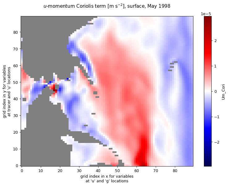
Let’s plot the Coriolis and pressure gradient contributions to the model -momentum budget on tile 7 (North Pacific). This is a rotated tile, which means the positive direction is southward. Hence the -momentum budget corresponds to approximately the meridional momentum budget, with the sign reversed.

import matplotlib as mpl
seismic_nanmasked = mpl.colormaps['seismic'].copy()
seismic_nanmasked.set_bad('gray')

plt.figure(figsize=(10,7), dpi= 90)
ds_u_mom.Um_Cori.isel(time=4,k=0,tile=7).plot(cmap=seismic_nanmasked)
plt.title('$u$-momentum Coriolis term [m s$^{-2}$], surface, May 1998\n')
plt.show()

plt.figure(figsize=(10,7),dpi=90)
ds_u_mom.Um_dPhiX.isel(time=4,k=0,tile=7).plot(cmap=seismic_nanmasked)
plt.title('$u$-momentum pressure gradient term [m s$^{-2}$], surface, May 1998\n')
plt.show()

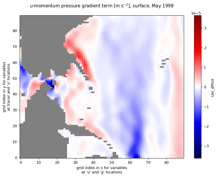
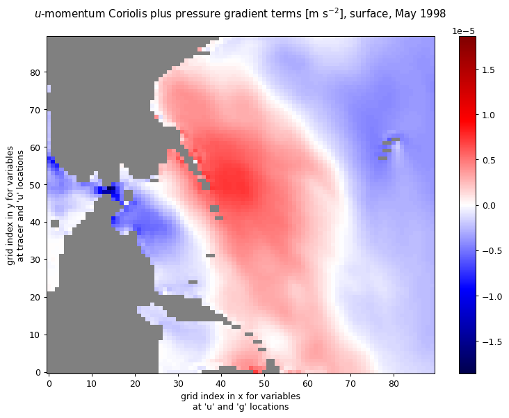
The fact that these two terms are nearly equal and opposite reflects the dominance of geostrophic balance. The sum of the Coriolis and pressure gradient terms (1st plot below) is balanced mostly by two frictional terms (2nd plot below): the sum of the surface (Ekman) stress included in the external forcing term Um_Ext, and the implicit dissipation of momentum Um_ImplD.

Um_Cori_plus_pgrad = ds_u_mom.Um_Cori + ds_u_mom.Um_dPhiX

plt.figure(figsize=(10,7),dpi=90)
Um_Cori_plus_pgrad.isel(time=4,k=0,tile=7).plot(cmap=seismic_nanmasked)
plt.title('$u$-momentum Coriolis plus pressure gradient terms [m s$^{-2}$], surface, May 1998\n')
plt.show()

Um_Ext_plus_ImplD = ds_u_mom.Um_Ext + ds_u_mom.Um_ImplD

plt.figure(figsize=(10,7),dpi=90)
Um_Ext_plus_ImplD.isel(time=4,k=0,tile=7).plot(cmap=seismic_nanmasked)
plt.title('$u$-momentum external forcing + implicit dissipation terms [m s$^{-2}$], surface, May 1998\n')
plt.show()

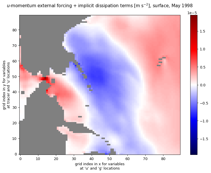
Notice that the two term combinations above are nearly equal in magnitude and opposite in sign.

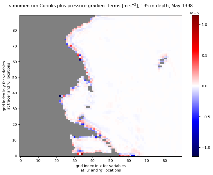
If we look at a level well below the surface (~200 m), the residual after summing the Coriolis and pressure gradient terms is even smaller.

k_plot = 16

plt.figure(figsize=(10,7),dpi=90)
Um_Cori_plus_pgrad.isel(time=4,k=k_plot,tile=7).plot(cmap=seismic_nanmasked)
# the syntax "%.0f" % X" rounds X to the nearest integer, with 0 digits after the decimal point
plt.title('$u$-momentum Coriolis plus pressure gradient terms [m s$^{-2}$], '\
            +f'{"%.0f" % -Um_Cori_plus_pgrad.Z[k_plot].values} m depth, May 1998\n')
plt.show()

Exercise: Try plotting the terms of the meridional momentum budget globally. To do this successfully you will need both the - and -momentum terms, and to interpolate and rotate them using the and parameters in the grid file (you can use the v4r4 grid file for this). This tutorial is a good resource for how to do the interpolation/rotation on the llc90 grid.